Economica

When referring to plaintiffs with normal mental capacity, the term “management fee” usually refers to expenses that plaintiffs incur for advice concerning investment decisions. Decisions concerning how their awards are to be spent – on medical care, accommodation, transportation, etc. – can generally be left to the plaintiffs themselves.

Plaintiffs who have suffered an impairment in their mental capacity – usually children injured at birth or adults injured in catastrophic accidents – however, may require assistance with many, if not most, of the decisions concerning expenditure of their awards. In this article, I propose to include the cost of this assistance in the term “management fee” and to investigate what the determinants of this fee will be in the case of plaintiffs with reduced mental capacity.

In the first section of this article, I enumerate the various types of assistance that will be required by these plaintiffs. I call this the “hierarchy of needs,” as the responsibility for this assistance involves a pyramid, or hierarchy, of decision-makers. In the second section, I investigate the costs of this assistance.

A Hierarchy of Needs

The management of the plaintiff’s award requires four types of agents:

Financial manager: Once the court award has been paid to the plaintiff, that amount will have to be invested. This will require either that a trust company invest the award in a portfolio of conservative financial assets, or that a structured settlement be purchased from an insurance company. In either case, a fee may be charged for the management of the plaintiff’s finances. (These are the fees that were discussed in the first article in this edition of the Expert Witness, “The Cost of Managing the Plaintiff’s Investments.”)

Guardian – The role of the guardian is to determine how the invested funds are to be spent: to ensure that the plaintiff is provided food, clothing, shelter, transportation, health care, and emotional care. Generally, it is not intended that the guardian will provide these services directly but will, instead, be responsible for hiring an agent called a case manager (see below), and for providing that individual with directions concerning the types and levels of services that are required. The guardian, for example, might decide that the plaintiff should be moved from his or her own home to a nursing home, but leave the decision about the selection of a specific nursing home to the case manager.

Often, the guardianship function will be performed by a committee which might, for example, include family members, legal representatives, social workers, and a life care planner/cost of care expert. The latter are experts who assist the guardian with the development and implementation of a plan for the care of the plaintiff.

Rehabilitation case manager – The guardian will often consider it necessary to contract with an agent to implement the plan that was developed in coordination with the life care planner. This individual is usually called a rehabilitation case manager, or simply case manager. He or she takes direction from the guardian and reports to the trustee (see below).

These individuals are responsible for:

the physical safety and emotional and social well-being of the individual in the community – for example, contracting with rehabilitation specialists, physical therapists, educational consultants, and speech and language consultants;
contracting with care personnel, such as rehabilitation assistants, home support workers, and nursing staff as warranted by the nature and extent of the injuries sustained and the impact of the impairments on functional ability; and
purchasing and maintaining goods and services, including medically-required equipment, such as wheelchairs and modifications to automobiles.
They are also responsible for monitoring all of the service-providers that have been hired, to ensure that their functions are being carried out as specified, and for replacing any employees who have resigned or been laid-off.

[As the case manager’s role is primarily to arrange for the purchase of goods and services, he or she may hire a subsidiary set of agents who make the actual purchases. Hence, there may be an additional layer of agents in the hierarchy: purchasing agents.]

Trustee: The trustee performs a “gatekeeping” role, ensuring that the bills incurred on behalf of the plaintiff are paid, that relevant income taxes are remitted, and that expenditures are not mismanaged (or misappropriated). Although one person (for example, a close relative) could act as both guardian and trustee, it is generally recommended that these two functions be separated, in order to provide independent checks on spending patterns.

Management fees

Payment may have to be made to each of the four categories of agents described above. I consider each of them separately here.

Financial Manager: As brain injured plaintiffs and children cannot make their own financial decisions, a third party will have to be employed to invest plaintiffs’ awards. Two options are available: a trust company may act as an investment manager, or an insurance company may provide a structured settlement.

If a trust company has been employed, it will provide its services for a fee that normally varies from about 1.0 percent to 2.0 percent of the value of the investment. Thus, for example, if the trust company is able to obtain a rate of return of 4.0 percent on the investment, from which it deducts a fee of 1.0 percent, the net rate of return will be 3.0 percent. Technically, the financial manager’s fee could be included as one of the costs of caring for the plaintiff. However, the data we recommend the courts use when calculating discount rates – the return on balanced portfolio funds (discussed in the first article in this edition of the Expert Witness,) – and the discount rates that are mandated by many provinces, are already net of investment companies’ management fees. Thus, in practice, no additional allowance will be required.

Similarly, insurance companies’ prices for structured settlements incorporate their costs of management. Hence, if the plaintiff’s award has been paid as a structured settlement, it may not be necessary to provide a separate allowance for the insurer’s management fee.

Note, however, that although it is generally not necessary to include a fee for the financial manager, it may be necessary to include a fee for the trustee (see below).]

Guardian/life care planner: There are three potential sources of guardians: the relatives of the plaintiff, a public agency (often referred to as the Public Trustee’s Office), or a private agent.

Relatives: When brain damage arises from negligence at birth, the parents of the injured child will often act as guardians; and when injury occurs later in life, guardians may be selected from spouses, parents, siblings, adult children, or other relatives. To the extent that these individuals are willing to work for free, it might be argued that no claim for their services can be made against the defendant. However, two counterarguments can be made.

First, for the same reason that relatives are often able to claim for the costs of providing household services or nursing care to the plaintiff, they may also be able to claim compensation for the time and effort required to act as guardians. Second, some allowance must be made for the possibility that the relative guardian will die before the plaintiff and, therefore, that a third party will be needed.

When either of these arguments is accepted, the cost of guardianship can be calculated as the cost that would have been charged by a public or private guardian. (For these, see below.)

Public Agency: Depending on the jurisdiction, Public Guardians may not charge fees for their services, or may charge a below-market fee. It should be noted, however, that all of the experts we have consulted have recommended that, if plaintiffs have large awards, they should not rely on the office of the Public Guardian, as the latter generally deals with relatively small sums.

Private Guardian or life care planner: If it is felt that the Public Guardian is not appropriate, it may be necessary to hire a private guardian. A number of knowledgeable individuals have suggested to me that a life care planner might fill this role. As the function of this individual is to develop a plan for the care of the plaintiff and to ensure that that plan is implemented as intended, it may require only a limited number of hours – perhaps five to ten per month – at approximately $200 per hour. Thus, an annual allowance of approximately $20,000 would not be unreasonable.

A guardian committee may also include a lawyer. If we assume five hours per month at $300 per hour, the annual fee would be $18,000.

Rehabilitation case manager: The costs of hiring rehabilitation case managers vary significantly depending on the severity of the injury to the plaintiff. A U.S.-based life care consulting firm, Caragonne and Associates, has developed an “assessment protocol” for calculating the number of hours of case management that will be required for seriously injured clients. The protocol identifies five dimensions of care, and scores each dimension on the degree of involvement required from the case manager: from low, through moderate, to high. The five dimensions are:

Level of client’s independence: This dimension measures the extent to which the client needs advice and encouragement. It ranges from high independence, in which the client requires only “periodic encouragement” from the case manager, to low independence/high need, in which frequent intervention is required to assist and orient the client.
Number of providers of needed services: This dimension ranges from low intervention, in which the client has obtained the resources needed, to high intervention, in which the case manager will have to contact multiple agencies and providers to arrange for the goods and services needed by the client.
Frequency of appraisal: The more often can the client’s status be expected to change, the greater will be the need for reappraisals by the case manager.
Coordination of providers: Once a life care plan has been put into place, the case manager will have to coordinate the implementation of that plan. The greater is the number of providers that have to be coordinated, and the more frequent is the number of interventions, the greater will be the number of hours worked by the case manager.
Travel: The further the case manager has to travel in order to meet with the client and his or her providers, the greater will be the number of hours required.

Caragonne and Associates estimate that if the client’s needs are rated as “high” on four or more of these dimensions, case management will require eight to twelve hours per month. If the client’s needs are rated as “moderate” on most of the dimensions, case management will require five to seven hours per month. Even a “low” rating on most dimensions will require one to four hours per month.

As many brain-injured clients and child plaintiffs will require a high level of services on most of the Caragonne dimensions, it can be expected that case management will require eight to twelve hours per month. Assuming ten hours per month, at $100 per hour, a case manager would cost approximately $12,000 per year.

Trustee: When trust companies act both as financial managers of the plaintiff’s award and as trustees of the plaintiff’s expenditures, they may offer a rate that is lower than the sum of the financial management fee and the trustee’s fee. As practices will vary among companies, it is important that counsel receive clear quotations for the sum of the two services.

If the Public Trustee acts as trustee, it may charge for its services. In Alberta, for example, that fee equals three-eighths of a percent of the total size of the investment – that is, $3,750 per year for each $1million.

When a structured settlement has been purchased from an insurance company, the insurer will not act as trustee. Hence, an additional fee for that service will often have to be calculated. RBC, for example, will act as trustee of a structured settlement for a charge of 5% of the annual annuity payment, subject to a minimum annual fee of $7,500. Tax preparation services would be in addition, at hourly rates, likely under $1,000/yr.

Summary

It has been our observation at Economica that when the courts use the term “management fee” they are usually referring to the fee for a financial manager, to supervise the investment of the plaintiff’s award. What I have argued in this article is that, when the plaintiff is a child or has been brain injured, there are at least three other classes of agents who will be responsible for managing the expenditure of the award, and who may also have to be compensated. In those cases, therefore, the “management fee” may extend well beyond the value normally considered by the courts.

Most importantly, allowance may have to be made for compensation of the guardian, the life care planner, and the case manager; and, when the award has been invested in a structured settlement, allowance may have to be made for trustee fees. As these fees could well exceed $50,000 per year, they could add over $1million to the size of the award to a young person. Hence, it is crucial that these sources of cost be considered seriously.

Christopher Bruce is the President of Economica; he has a PhD in economics from the University of Cambridge

The Cost of Managing the Plaintiff’s Investments

Posted on December 11, 2018December 11, 2018 By economica

As most individuals are unaccustomed to managing large sums of money, it may be appropriate for plaintiffs to employ advisors to assist them with the investment of their awards. In these cases, it has often been argued that the cost of hiring such advisors should be added to the value of the award. This cost is referred to as a management fee or financial management fee.

The fees that are charged by financial advisors are almost universally quoted as a percentage of the total value of the amount that has been invested. For example, the fee charged by a bank or trust company for managing an investment of $1 million might be 2.0 percent of that investment, or $20,000 per year. This percentage normally declines as the size of the investment increases. For example, on an investment of $3 million, it might be 2.0 percent on the first $2 million and then 1.5 percent on the next $1 million.

The effect of the management fee is to reduce the net value of the rate of interest, or discount rate, obtainable by the plaintiff. For example, assume that a trust company is able to obtain a rate of return of 5.0 percent (after accounting for inflation) on an investment of $1 million, and that the management fee is 2.0 percent. The income earned in each year will be 5.0 percent of $1 million, or $50,000. But from that will be deducted a 2.0 percent management fee, or $20,000. Thus, the net return on the investment will be $30,000 ($50,000 – $20,000), which represents a 3.0 percent net rate of return on the investment.

When calculating the value of the plaintiff’s award, the financial management fee could be taken into account either by adding the dollar cost of the financial advisor to each year’s losses, or by discounting the future losses by the net rate of return on investments. The former approach requires the calculation of the management fee for each year in the future, whereas the latter requires only that the rate of return on investments be replaced by the net rate of return (3.0 percent is used in the example above instead of 5.0 percent). Thus, as both approaches produce the same estimate of the award, economists generally prefer to use the simpler approach: the net rate of return.

Assume that it has been agreed that plaintiffs should place their awards in a particular type of investment portfolio, and that the projected rate of return on that portfolio is, say, 4.5 percent. If the financial management fee is 1.75 percent, the appropriate discount rate would be 4.5 percent minus 1.75 percent, or 2.75 percent.

This is the basis of the argument that is often made in court: that a (financial) management fee must be deducted from the discount rate to obtain a “true” net discount rate.

Although this argument sounds reasonable, it is not – for the simple reason that in most cases in which financial experts testify concerning the value of “the discount rate”, it is a net discount rate to which they are referring. That is, they are referring to a rate from which the management fee has already been deducted. Thus, it is not necessary to deduct a further management fee from the recommended discount rate – the latter already includes a management fee.

What I wish to show in the following two sections is that whether it is necessary to deduct the management fee will depend upon the way the discount rate has been determined.

In the first of these sections, I will consider four situations in which the court has used testimony from expert witnesses to select the discount rate. In the second section, I will consider those cases in which the discount rate has been mandated by government regulation.

Court Selected Discount Rate

The courts have been clear that plaintiffs are expected to invest their awards in financial assets that do not expose them to unreasonable risk. For example, in its seminal decision in Lewis v. Todd (1980 CarswellOnt 617), the Supreme Court of Canada approved of the expert’s use of “high grade investments [of] long duration.” [para. 17] Financial experts have generally held that this implies that the plaintiff’s award should be invested in a balanced portfolio of conservative financial assets – for example in a mix of government bonds, highgrade corporate bonds, and “blue chip” stocks.

In this section, I will consider four approaches that plaintiffs could take to the investment of their awards; and investigate whether it would be appropriate to deduct a management fee in each of them. These approaches assume that the plaintiff will either:

Purchase mutual funds that spread their investments across balanced portfolios of financial assets.
Employ a financial advisor to assist them with decisions concerning their investments.
Use their own expertise to invest in financial markets.
Purchase a structured settlement.

Under the first three of these approaches, I assume that the plaintiff, and his or her advisors, will attempt to balance two goals: maximize the rate of return on investments, and minimize the risks associated with the purchase of financial assets. This balance is achieved by investing in a balanced portfolio of assets spread across a range of potential instruments. (Under the fourth, structured settlement approach, the plaintiff leaves the choice of investments to the provider of the structured settlement.)

Balanced portfolio funds: One method of achieving a balanced portfolio is to purchase a type of mutual fund called a balanced portfolio fund. Each of these funds – which are offered by all of Canada’s banks, by many investment houses, and by insurance companies – invests in a balanced blend of asset classes. These funds offer numerous advantages to the plaintiff. They reduce risk by spreading their investments across different types of assets, in different industries, and different countries. They offer clearly identified choices concerning the degree of risk that the plaintiff is willing to accept, often ranging from “very conservative“ to “aggressive growth-oriented”, and the selection of the assets to be incorporated in each fund is made by experts who are supported by teams of researchers.

Furthermore, balanced portfolio funds offer the attractive feature that the rates of return that they have earned are publicly available. Thus, not only can the plaintiff-investor determine easily what any fund’s performance has been; but the rates of return on those funds can be used by the courts as objective measures of the returns that are available to plaintiffs when they invest in conservative, balanced portfolios.

The interest rates that are reported publicly, on balanced portfolio funds, are net of management fees. For example, if a fund earns 4.5 percent on its investments, and the fund’s operators charge a fee of 2.0 percent, the published rate will be 2.5 percent. It is information concerning these published rates – that is, rates that are net of the fund operators’ rates – that Economica uses when discounting plaintiffs’ future losses. [See Selecting the Discount Rate, Expert Witness, Vol. 21, Spring 2017.] As these rates are net of the operators’ fees, there is no need to add a “management fee.”

Financial advisor: Instead of purchasing a mutual fund “off the shelf,” the plaintiff could employ a financial advisor to purchase a balanced portfolio of investments, specific to the preferences of the plaintiff. Generally, these advisors charge a fee that equals approximately 1.0 to 2.0 percent of the value of the assets that they are managing. Is there an argument for adding the cost of this advice to the plaintiff’s award, as a management fee? I will argue that the answer is “no.”

To see why, consider the following example: assume that a financial advisor who charges a management fee of 2.0 percent is able to obtain a rate of return of 5.0 percent. The net rate of return received by the advisor’s clients will be 3.0 percent. [For example, $100,000 invested at 5.0 percent will generate a return of $5,000 per year and, with a management fee of 2.0 percent, will cost $2,000 per year. Thus, there is a net gain of $3,000, which is 3.0 percent of the invested amount.]

In this case, the appropriate discount rate will be the net rate of interest obtained by the advisor, or 3.0 percent. For example, to determine how much would have to be invested today to replace a $103,000 loss a year from now, one would divide $103,000 by 1.03 (= 1 + the interest rate), to get $100,000. When future losses are discounted by this rate, the costs of the advisor’s services have been accounted for in the calculation – the $3,000 gain after one year equals the return on the investment, $5,000, minus the advisor’s fee, $2,000.

Thus, if the discount rate that is used by the court to calculate the value of the plaintiff’s award equals the net investment return obtainable by the financial advisor, no additional allowance needs to be made for a management fee.

Although the rates of return obtainable by financial advisors are not publicly available, a reliable objective measure of that rate is the rate of return on balanced portfolio funds. As
independent financial advisors generally rely on the same research that is available to the operators of mutual funds (they usually work for the same financial institutions), they can be expected invest in portfolios of financial assets that are similar to those that are contained in balanced portfolio funds. They can, therefore, be expected to generate similar rates of return net of management fees.

If that is true, then the estimate of the return available to independent advisors includes an allowance for the management fee, and no additional management fee need be awarded.

Self investment: In those cases in which plaintiffs are expected to use their own skills to invest their awards, there will be no (or only minor) management fees and, hence, no call for such fees.

Structured settlement: The cost of any structured settlement includes the cost to the issuer of managing that settlement. Hence, again, there would be no need for an additional management fee.

Summary: I can find no situation in which it would be necessary to award a management fee to a plaintiff who is mentally competent.

Mandated Discount Rate

An argument might be made for the award of management fees in those cases in which the discount rate mandated by the government exceeds the rate predicted by the experts before the court.

Assume, for example, that the mandated rate was 3.0 percent and that the best evidence before the court was that the net rate of return available on a balanced portfolio of funds was 2.0 percent. It could be argued that the difference between the two rates had arisen because the mandated rate reflected the rate of return available before deduction of management fees. In that case, it might be appropriate to award a management fee of 1.0 percent, to bring the net discount rate to 2.0 percent.

It must be pointed out, however, that the rates currently mandated in British Columbia, Ontario, and Saskatchewan are significantly lower than the net rates available on balanced portfolio funds. Hence, although there is a case for awarding management fees in some cases, the conditions for those cases do not exist at this time.

Conclusion

In virtually every situation in which financial experts testify concerning the value of the discount rate, the rate of return that they refer to is net of the cost of investment. Hence, it is not necessary to deduct a financial management fee. And, although such a deduction might be necessary in cases in which a mandated discount rate had been used, the rates that have been mandated in Canada in recent years are so low that it must be concluded that they are also net of management fees.

Christopher Bruce is the President of Economica; he has a PhD in economics from the University of Cambridge

Admissibility of Expert Evidence: Personal Injury Litigation

Posted on December 11, 2018 By economica

The admission of expert evidence has required that the courts maintain a fine balance between, on the one hand, caution against the possibility that witnesses may usurp the court’s role of forming opinions and drawing conclusions; and, on the other hand, recognition of the fact that juries and triers of fact may lack the technical expertise to draw inferences from the facts as presented.

This dichotomy has led the courts and legal commentators to develop a lengthy set of principles concerning the admissibility of experts and their evidence. These principles can usefully be divided into four categories: the requirement that expert testimony be useful; the identification of whether the expert is qualified; the determination of whether the expert’s testimony is reliable; and the evaluation of the weight that is to be attached to the expert’s opinion.

In this article, I summarise some recent rulings in Canadian and American law with respect to each of these categories. I find that although it is rare in western Canada for the courts to disqualify a witness who has been tendered as an “expert,” there are many instances in which the court will accept a witness’ qualifications subject to the understanding that opposing counsel will exercise its right to subject the witness to vigorous crossexamination. And in many others, the court will caution that an expert’s testimony is to be given reduced weight.

1. Useful
The first requirement that must be met before an expert can be permitted to testify – often referred to as the “gatekeeper” component – is that the expert’s testimony must be shown to be “necessary in assisting the trier of fact.” (R. Mohan, [1994] 2 S.C.R. 9). This requirement has a number of implications.

First, the expert’s testimony must not have the effect of usurping the court’s function, of weighing evidence, evaluating the credibility of witnesses, making findings of fact, reaching conclusions concerning legal matters, etc. In Snelgrove, (2015 ONSC 585, at para 12), for example, the court disqualified a witness, in part because he “…purports to come to legal conclusions,” specifically concerning the defendant’s intent, negligence, misrepresentations, and misconduct.

Second, the expert’s report must offer an opinion concerning the issues in dispute. See, for example, Hoang v Vicentini (2012 ONSC 1358) in which an accident reconstruction expert’s report was dismissed on this ground.

Third, for expert evidence to be admissible:

[t]he subject matter of the inquiry must be such that ordinary people are unlikely to form a correct judgment about it, if unassisted by persons with special knowledge. (Kelliher (Village of) v. Smith, [1931] S.C.R. 67 quoting from Bevan on Negligence)

Or, as Lawton, LJ concluded in R. v. Turner ([1975] Q.B. 834, at 841):

An expert’s opinion is admissible to furnish the court with scientific information that is likely to be outside the experience and knowledge of a judge or jury. If on the proven facts a judge or jury can form their own conclusions without help, then the opinion of an expert is unnecessary.

In Canada, there has been little debate about the definition of the term “scientific information” as used in Turner. In the United States, however, two decisions of the Supreme Court – Daubert v. Merrell Dow Pharmaceuticals, Inc ((1992) 509 U.S. 579) and Kumho Tire Co. v. Carmichael ((1999) 131 ) – have ruled on the interpretation of the terms “scientific, technical, or other specialized knowledge” contained in Rule 702 of the U.S. Federal Rules of Evidence. Of particular importance to Canadian practitioners is that the Supreme Court of Canada, in R. v. J.-L. J. ([2000] 2 S.C.R. 600, 2000 SCC 51) explicitly approved of the four criteria set out in Daubert for determining whether expert testimony met the requirement that it constitute “scientific knowledge.” These are:

Whether the theory or technique “can be (and has been) tested”.
Whether the “theory or technique has been subjected to peer review and publication”.
In the case of a particular technique, what “the known or potential rate of error” is or has been.
Whether the evidence has gained widespread acceptance within the scientific community.

The Daubert criteria proved less applicable to issues involving “technical” than “scientific” knowledge, such as that often proffered by engineers, however. Accordingly, the United States Supreme Court agreed to hear Kumho Tire. In that case, an expert in tire failure analysis relied in part on his own (extensive) experience to determine whether a failure in a tire was caused by a defect and not by misuse on the part of the plaintiff. As the expert’s testimony did not meet any of the criteria set out in Daubert, the issue in Kumho was whether “technical and other specialized knowledge,” as defined in Rule 702, was to be subjected to the same criteria as was “scientific knowledge.”

The Court ruled that it was not. Testimony about a technical matter could be considered to be “expert” if it:

…focuses upon specialized observations, the specialized translations of those observations into theory, a specialized theory itself, or the application of such a theory in a particular case.

The function of Rule 702 was not to restrict expert testimony to a narrow set of “scientific” disciplines, but to:

… make certain that an expert, whether basing testimony upon professional studies or personal experience, employs in the courtroom the same level of intellectual rigor that characterizes the practice of an expert in the relevant field.

It was the application of “intellectual rigor” that distinguished an expert from a layman, as much as did the possession of specialised, formal training.

2. Qualified
As the expert’s role is to provide information that is not within the “experience and knowledge of a judge or jury,” it is necessary to show that those individuals who are presented as “experts” possess the requisite training and experience. With respect to scientific knowledge, this has generally meant that the witness must have obtained a graduate degree, such as an M.Sc. or Ph.D., or a professional designation, such as a law or accounting degree. With respect to technical skills, an individual (such as the tire expert in Kumho) may develop “expertise” through long personal experience with the matter before the court. In both cases, however, the witness is expected to apply intellectual rigour to the interpretation of the evidence before the court.

Furthermore, the expert’s testimony may not be admitted if his or her qualifications are inferior to those of other witnesses who have been tendered as experts in the same action. It was for this reason that, in Levshtein v Ramirez (2013 ONSC 521), a chiropractor’s opinion concerning the plaintiff’s ability to perform household tasks was not admitted. Although the chiropractor had performed a number of tests of the plaintiff’s hand strength and weight-lifting ability, the court found that other witnesses were more qualified to testify concerning the extent to which the plaintiff’s physical disabilities had affected his activities in the home.

In a recent survey of more than 12,000 American decisions, PWC (formerly Price Waterhouse Cooper) found that the courts had focussed on two factors: relevant academic credentials and relevant experience, when evaluating qualifications. The courts generally ruled that extensive experience might be sufficient to outweigh lack of credentials (for example, working as an bookkeeper in a role relevant to the case, such as franchising); and appropriate credentials might not be enough if the area of specialization was not relevant (for example, an expert testifying on loss of earnings might have a PhD in economics, but in international trade). (PWC, Challenges to Financial Experts: 2000-2016, (pwc.com).)

3. Reliable
Two broad issues are canvassed when determining whether the testimony of the expert is of sufficient reliability to be of value to the court. First, the evidence presented by the expert must be “relevant;” that is, it must be “… so related to a fact in issue that it tends to establish it.” (Mohan, at 20) Second, the expert must provide an “objective and unbiased” opinion.

Relevant

To be relevant, expert evidence must meet two criteria. First, any factual evidence must meet standard tests of statistical reliability. Data must be collected in a manner that ensures that it is representative of the group to which it is to be applied. For example, if a doctor’s opinion is based on observation of his or her own patients, precautions must be in place to ensure that those patients are similar to the plaintiff in question. Similarly, if evidence is drawn from reports published by third parties, the expert must be careful to ensure that the definitions used in those studies refer to the same concepts that are of importance to the case at hand. [For further elaboration on these points, see Christopher Bruce, “The Reliability of Statistical Evidence Concerning the Impact of Disability” The Expert Witness, 2004 (3).]

Second, there must be a compelling logical and/or statistical correlation between the evidence that has been presented and the conclusion that the expert purports to draw. This is particularly problematic when the expert misunderstands or misrepresents statistical studies that have been published by third parties.

Objective and unbiased

If an expert has a financial, personal, or professional interest in the outcome of a case, which may induce that expert to bias his or her opinion, the court may either disqualify the expert or place reduced weight on that opinion. [The following discussion is informed largely by the decisions in United City Properties v. Tong, 2010 BCSC 111 and R. v Klassen, 2003 MBQB 253; and by Paul Michell and Renu Mandhare, “The Uncertain Duty of the Expert Witness,” Alta L Rev 42.3 (2005).]

Financial: A number of factors have been identified by the courts that may have led the expert to have a financial interest in the outcome of the case. These include:

A contingency fee,
A long association, or exclusive association, with one lawyer or party,
Employment by either the plaintiff or defendant.

Personal: The witness’s objectivity may also be questioned if he or she had:

A personal interest in the outcome, either because that outcome would directly affect the witness or because it would set a precedent that would affect him or her,
A personal relationship, such as friendship or a family connection, to one of the litigants.

Professional: If the witness has taken a strong stance on a contentious issue facing the courts – such as the manner in which the discount rate is to be determined – that witness may come to consider his or her professional reputation to be dependant on acceptance of that view by the court. This may lead the expert to discount or ignore evidence contrary to his or her professed view.

Even in the absence of evidence that an expert has an interest in the outcome of the case, the court may still find bias, based on the content of the expert’s statements, report, or testimony. Evidence of such bias has been found when:

The witness has been found to have made statements publicly that show philosophical hostility towards certain subjects,
The expert’s report has been withdrawn or modified without reasonable explanation,
The expert’s opinion has been found to differ, for unexplained reasons, between occasions on which the expert appeared for the defence and those when he/she appeared for the plaintiff,
The expert has departed from any governing ethical guidelines established in the expert’s field of expertise,
The expert has persistently failed to recognize other explanations or to provide a reasonable range of opinion,
The witness has operated beyond his or her field of stated expertise, such as when an economist comments on the appropriate costs of caring for an injured plaintiff,
The expert has failed to substantiate his or her opinions,
The expert has acted as an “…informed champion or enthusiastic supporter of the retaining party’s cause.” (Michell and Mandhare at 648, quoting Halpern v. Canada (A.G.) (2002), 215 D.L.R. (4th) 223 at paras. 143-44 (Ont. Div. Ct.).)

Nevertheless, in Moore v Smith Construction (2013 ONSC 5260), a scientist who worked for an advocacy group that provided legal services to the respondent was allowed to testify as an expert. The court found, following a voir dire, that there was no evidence of bias or partiality. Instead of disqualifying the scientist, the court ruled that the “… fact that the proposed expert is employed by the party can be taken into account when the trial judge assesses the weight and value of the evidence”. (at para 47)

4. Weight

If the court has found a degree of bias in the expert’s testimony, it can choose among: disqualifying the expert, announcing that it will allow the expert’s testimony but give lesser weight to that evidence, or leaving criticism of the expert’s report to cross-examination by opposing counsel.

Of these, the first would seem to be of primary importance in cases that were tried before a jury, and the second and third to cases that were heard before a judge. As a judge will, presumably, be less influenced by biased and unqualified witnesses than would be a jury, it may be less harmful to permit questionable testimony when the case was being tried by judge alone than when it was being heard before a jury. On these grounds, we would expect experts to be disqualified more often in Canadian courts in criminal cases than in tort cases; and more often in tort cases in the United States than in equivalent cases in Canada.

In Gutbir v University Health Network (2010 ONSC 6394), a medical malpractice case, the court allowed the treating physician to testify to fact; but, on the ground that he had a personal interest in the outcome of the case, it denied him qualification as an expert.

Contrary to our speculation above, however, the PWC survey found that American courts are reluctant to exclude expert testimony. Rather they apply a “light hand on the gate”, preferring to subject the expert’s opinion to vigorous cross-examination, especially if the disagreement concerns the choice of an appropriate or inclusive set of data. They were also found to be willing to allow experts to revise their reports in light of objections from opposing counsel.

Summary

The courts admit the testimony of expert witnesses only with a good deal of apprehension. First, they are reluctant to cede their role of weighing evidence, evaluating the credibility of witnesses, making findings of fact, reaching conclusions concerning legal matters, etc. And, second, they have qualms about the qualifications and independence of witnesses who have been tendered as “experts”.

As a result, the courts have developed lengthy lists of requirements that witnesses must meet before they can be accepted. The purpose of this article has been to review these requirements and to ask how they have been applied in practice. The most important finding of this review has been that the requirements have become sufficiently well known that it is uncommon for legal counsel to put forward individuals who fail to meet the court’s assessment. Rare cases remain in which experts are disqualified; but, more commonly, where an expert has been challenged, the court has allowed the expert: to re-write his or her report, to submit the report subject to the condition that it will be given reduced weight, or to testify subject to the understanding that opposing counsel has the right to cross-examine “vigorously”.

Christopher Bruce is the President of Economica and a Professor of Economics at the University of Calgary.

Selecting the Discount Rate (2017)

Posted on May 11, 2017May 30, 2017 By economica

by Christopher J. Bruce, Derek W. Aldridge, Kelly Rathje, Laura Weir

When calculating the lump sum award that is to replace a stream of losses in the future, it is first necessary to determine the rate of interest, or discount rate, at which the award will be invested. In Canada, this rate is set equal to the real rate of interest, that is, to the nominal (or “observed”) interest rate net of the rate of inflation.¹

Whereas most provinces mandate the discount rate that is to be used when calculating the present value of future losses, Alberta has left the determination of that rate to the courts. Accordingly, the testimony of financial experts on this matter has become an important element of most personal injury actions.

Over the last forty years, Economica has made important contributions to the debate concerning the choice of a discount rate. These contributions have come in the form of chapters in our textbook, Assessment of Personal Injury Damages (now in its fifth edition), articles in this newsletter, and submissions to reviews of the mandated rates in Ontario, Saskatchewan, and British Columbia.

In this article, we argue that whereas virtually all financial experts (including ourselves) have implicitly applied what we will call here the active management approach to the determination of the discount rate, it can be argued that an alternative technique, which we will call the annuity approach, is often more appropriate.

In Section I of this article, we describe these two approaches and investigate their relative merits. In Section II, we employ the principles developed in the first section, to examine how numerical measures of the discount rate might be obtained when discounting two types of future costs: medical expenses and losses of earnings. Finally, in Section III, we summarise our findings.

In that Section, we argue that:

if the plaintiff chooses to self-manage the investment of his or her award, the appropriate discount rate (net of inflation) is 2.5 percent; whereas
if the plaintiff chooses to purchase a life annuity, or have the defendant purchase a structured settlement, the appropriate discount rate (net of inflation) is zero percent. We argue that it is to the advantage of plaintiffs to make this choice in most cases in which their losses are expected to continue into ages of high mortality (usually after age 75 or so).

I. Two Approaches to Selecting the Discount Rate

There are two broad approaches to the determination of the discount rate, the annuity approach and the active management approach. In the former, it is assumed that plaintiffs will use their lump sum awards to purchase annuities. In the latter, it is assumed that they will invest their awards in a portfolio of stocks, bonds, mutual funds, and other financial assets.

In this section, we define the two approaches and investigate their relative merits. We conclude by identifying the circumstances in which each approach might be preferred to the other.

1. The Two Approaches Defined

The Annuity Approach

If the plaintiff has been awarded a lump sum award to replace a stream of losses from the date of trial until some specified termination date – most often the plaintiff’s projected date of retirement or date of death – he or she will be able to replace the future losses by purchasing an annuity, usually from a life insurance company. This purchase can take the form of either a life annuity or, under the auspices of the court, a structured settlement. In either case, the plaintiff will receive a specified stream of benefits until the termination date.

The purchase price of the annuity will be determined by three main factors: the value of the annual payments, the number of years to the termination date (which will, in part, be determined by the life expectancy of the plaintiff), and the rate of interest at which the insurance company is able to invest the funds received from the plaintiff (or defendant, in the case of a structured settlement).

It is this rate of interest that is known as the discount rate. In the case of an annuity, the discount rate is determined primarily by the requirement (arising both from regulation and accepted accounting practices) that the stream of payments the insurance company has contracted to make is matched by the stream of income that the company will receive from its investment. That is, at the time the annuity contract is signed, the insurance company will invest a sufficient amount, in secure financial instruments, that the income generated from that investment will be sufficient to fund the stream of payments the company has contracted to pay.

What this implies is that for each promised future payment, the insurance company will, implicitly make a separate investment that will generate sufficient returns that it will be able to cover the contracted payment at the appropriate date. For example, if it has contracted to pay $50,000 per year for ten years, it will make ten separate investments, each of which has a maturity value of $50,000.

The discount rate applicable to the payment that must be made one year from now is the interest rate currently available on one-year investments (such as one-year bonds); the rate applicable to the payment to be made two years from now is the interest rate currently available on two-year investments; etc. Thus, there could, in principle, be as many discount rates as there are time periods in the plaintiff’s stream of losses. (In practice, however, investments for more than ten or fifteen years tend to have the same interest rate, so a thirty-year annuity might require ten discount rates.)

Note, first, that there is not “a” discount rate. Rather, there is one rate for each year over which the stream of payments is to be made into the future.

More importantly, note also that it is not necessary to “predict” the discount rate(s). As the investments are to be purchased today (i.e. at the date of settlement), it is the interest rates that are available today that are to be used – and these rates are readily available.

Structured settlement: If it is assumed that a structured settlement is to be purchased, the argument concerning choice of a discount rate is similar to that for a life annuity. Again, the insurance company will place the lump sum received from the defendant in a series of investments, each of which will mature on the date that the payment is due. As the insurance company can be expected, once again, to purchase secure investments, the rates of return that are currently available on such investments can be used to determine the discount rate(s).

The Active Management Approach

Alternatively, the plaintiff might use his or her award to purchase a mixed portfolio of financial assets – for example, stocks, bonds, and mutual funds – selling and buying components within that portfolio as changes occur in financial markets. Because the individual is continuously selling old investments and purchasing new ones, the returns on those investments will reflect rising (and falling) rates that are available in the financial markets.

The complication that this approach introduces is that the rates of return that will be available at the times the plaintiff reinvests his or her funds are not known at the time that the court award is made. These rates must be predicted – in contrast to the rates employed in the annuity approach, which are known at the time the award is made.

2. Comparison of the Two Approaches

As the plaintiff’s award is intended to replace an ongoing loss, it is important that the income the plaintiff receives from investment of that award is sufficient, in each period, to provide the desired compensation. In turn, this requires that the rate of return on that investment be as predictable as possible. The less predictable is the rate of return, the less certain can the courts be that the award will be sufficient for its purposes.

The predictability of the rates of return obtained under the annuity and active management approaches differs with respect to three characteristics: volatility of the rate of return on the invested funds, uncertainty concerning the plaintiff’s life expectancy, and protection against unanticipated increases in the rate of inflation. In this section, we compare the two investment approaches with respect to each of these characteristics in turn.

Volatility

The volatility of a class of investments refers to the variability in the rate of return earned on those investments over time. According to one source:

… volatility refers to the amount of uncertainty or risk about the size of changes in a security’s value. A higher volatility means that a security’s value can potentially be spread out over a larger range of values. This means that the price of the security can change dramatically over a short time period in either direction. A lower volatility means that a security’s value does not fluctuate dramatically, but changes in value at a steady pace over a period of time. [investopedia.com, emphasis added]

The more volatile is the price of a security, the more likely it is that the rate of return on that security will deviate from its long run average. In some periods the return will rise above the average and investors will experience a windfall; but in other periods, the return will fall below average and investors will experience a shortfall.

In the very long run, high returns and low returns may average out, and the rate of return obtained will trend towards the long run value. However, many plaintiffs do not invest for a period long enough that they can be confident that the rate of return on investment of their awards will settle on the long run average. This will particularly be true if plaintiffs are unlucky enough to make a major investment shortly before markets enter a sharp downturn such as was experienced in 2008, (or lucky enough to invest shortly before an upturn, such as in 2010).

To avoid the uncertainty that may result if the plaintiff’s award is invested in volatile financial instruments, it is often recommended that they concentrate their investments on secure, non-volatile stocks, bonds, and mutual funds. The Canadian courts have confirmed this recommendation. For example, in its seminal decision in Lewis v. Todd (1980 CarswellOnt 617), the Supreme Court of Canada approved of an expert witness’s use of “high grade investments [of] long duration.” [para. 17]

Investments in life annuities offer the lowest volatility possible: essentially, the rate of return is guaranteed as long as the insurer, and its re-insurers, remains viable.

Investments in an actively managed portfolio experience two forms of volatility that are not found with annuities. First, all but the most conservative, high grade investments experience variations in returns from year to year.

Second, even if a sophisticated investor could avoid most year-to-year variations in the rate of return, no investor can protect him- or herself against variations that occur due to long-term changes in the economy. For example, assume that it had been anticipated that the plaintiff would be able to obtain a two percent rate of return on investment of his/her award, because the economy was expected to grow at that rate. If broad economic fundamentals should change, such that long run growth fell to one percent per year, it is unlikely that the individual investor would be able to maintain a two percent return on investments.

To conclude, if the goal is to minimize volatility in the returns on the plaintiff’s investments, life annuities and structured settlements are superior to active management, especially in the long run. For short periods of time, perhaps five or ten years, an actively managed “portfolio of high grade investments” may offer almost as much security as an annuity.

Life Expectancy

Assume that a plaintiff will require medical expenses of $50,000 per year for the rest of his life. In a personal injury action, his award will be calculated to ensure that if he invests that amount in a fund composed of secure investments, it will provide $50,000 per year for the lifetime of the average Canadian of his age and sex. For example, if he is a 50-year-old Canadian male his life expectancy is approximately 31 years, to age 81. Thus, his award will be calculated to ensure that he can remove $50,000 per year until his age 81, at which point the award have been drawn down (approximately) to zero.

This puts the plaintiff in a quandary: that the life expectancy of 50-year-old males is 31 years implies that (approximately) half of 50 year old males will live longer than 31 years (and half less than that). Thus, if the plaintiff spends $50,000 per year on medical expenses there is a 50 percent chance that his investment fund will be exhausted before he dies.

Alternatively, if he spends less than $50,000 per year, to leave money in the fund for the possibility that he will live beyond age 81, he will have insufficient funds in every year to pay for his required expenses. Even if it happens that the plaintiff lives less than 31 years, he will have been inadequately compensated for his necessary expenses, because he will have been taking the (reasonable) precaution of spending less than $50,000 per year to create a buffer for the possibility he will live longer than average.

In short, if plaintiffs invest their awards in actively managed investment funds, it is virtually certain that their awards will be insufficient to compensate them fully.

Furthermore, it can easily be shown that this outcome also arises when the amount to be replaced is a loss of income – although the shortfall will be less in this case than in the case of most medical expenses, because the impact of mortality is much lower when the loss continues only to retirement ages (when mortality rates are still low) than when it continues to the end of life.

If the plaintiff’s award is placed in a life annuity or structured settlement, however, payment of the desired annual compensation will be guaranteed from the date of settlement to the end date of the compensation period.

In short, whereas a life annuity will pay the plaintiff an amount equal to his or her loss in every year, an award invested in a portfolio of funds will, in most cases, undercompensate the plaintiff. This under-compensation will often be less when the award is intended to compensate for a loss of earned income than when it is to compensate for long term costs of care. Thus, on this ground, life annuities are slightly preferred to mixed portfolios of investments when there has been a loss of earnings; but annuities are definitely preferred when there is a long-term requirement for payment of medical expenses.

Unanticipated Inflation

A drawback to the annuity approach is that the stream of income that it provides may prove to be inadequate if inflation rates rise unexpectedly. For example, if an annuity provided for $10,000 per year, increasing each year at two percent (to allow for anticipated inflation), it would pay $12,190 in year ten. But if inflation proves to be four percent per year, the plaintiff will require $14,800 in year ten to buy what $10,000 would have bought in year one. The annuity will pay $12,190 when $14,800 is required.

It is often possible to buy annuities whose annual payouts increase with the actual rate of inflation. However, as the risk facing the sellers of annuities is quite high in this case, the price of these annuities may be higher than many buyers are willing to pay.

An alternative method of protecting against the effect of unanticipated inflation is to invest in an actively managed portfolio of assets. Under this approach, the individual is assumed to buy and sell financial assets on a continuing basis, replacing low-earning assets with higher-earning ones as market conditions change. If inflation increases, so will the returns on investments, particularly bonds, allowing the plaintiff to maintain a real rate of return (i.e. a rate net of inflation) that is consistent over time.

On this ground, if the rate of inflation cannot be predicted easily, the active management approach may be preferred to the annuity approach. However, central banks around the world have become convinced that one of their primary functions is to maintain a steady, low rate of inflation. The Bank of Canada, for example, has successfully targeted a rate of two percent since the early 1990s. This policy has been so well received that virtually all financial analysts expect this rate to be maintained well into the future.

As there is no reason to expect that the future rate of inflation will deviate significantly from the rate that has been experienced for the last twenty years, there is little reason to base the selection of the investment approach on the need to protect against unanticipated changes in the rate of inflation.

We conclude, therefore, that the ability of the active management approach to provide protection against unanticipated inflation does not offer a compelling reason to choose that approach in preference to the life annuity approach.

3. Summary

We summarise this section by investigating the merits of using the two investment approaches to replace (i) costs of medical care and (ii) losses of earnings.

Costs of Medical Care

For two reasons, if the plaintiff’s award is intended to provide compensation for medical expenses, particularly expenses that extend well into the future, we recommend that the award be invested in a life annuity (or structured settlement). First, as medical expenses are often required for the plaintiff’s entire life, it is important that the award is able to provide benefits should the plaintiff live beyond the average life expectancy. Whereas this can be achieved easily using a life annuity, it cannot be done through the active management approach.

Second, as the requirement for medical expenses often extends many decades into the future, the returns on awards invested in actively managed funds may be subjected to significant volatility, hence placing the risk of inadequate compensation on the plaintiff. The returns on a life annuity, however, are guaranteed by the insurer, thereby removing the risk of volatility from the plaintiff.

The contrary argument, for using the active management approach to the funding of future medical expenses, is that this approach allows for protection against unanticipated inflationary changes. We have argued, however, that such changes are not expected to be so large as to counter the arguments for use of life annuities. Furthermore, if the courts decide that inflation is likely to become an important factor, they can require that plaintiffs purchase inflation-protected life annuities.

We conclude that, in most cases, it should be assumed that when the plaintiff’s award is to provide for medical expenses, it will not be invested in actively managed funds but will, instead, be used to purchase life annuities. The exception occurs when medical expenses are required for only a short period of time.

Loss of Earnings

When the purpose of the plaintiff’s award is to replace a future stream of lost earnings, the argument in favour of life annuities is weaker than it was with respect to medical expenses. The reason for this is that earnings losses will generally end at an age at which the annual rate of mortality is still quite low.

For example, as we argued above, if a 50-year-old man has a life expectancy of 81, there is (approximately) a fifty percent chance that he will live beyond that age and will exhaust any award for medical expenses. Assume, however, that that individual had planned to retire at age 60, bringing any loss of earnings to an end at that age. As the probability of dying before age 60 is very small, the difference between an award that allowed for that probability and one that did not would also be small. Thus, any “error” that arose from using the active management approach might be compensated by other factors.

If we assume again that the risk of unexpected changes in inflation is small, then the primary difference between the annuity approach and the active management approach (with respect to losses of earnings) will arise with respect to volatility. On this basis alone, the annuity approach will be preferred as it offers less risk that an unanticipated fall in interest rates will leave the plaintiff’s award inadequate.

However, it is possible that this uncertainty concerning the rate of return on investments might be offset if the active management approach provided higher average rates of return. For example, if those rates were two or three percentage points higher than those offered by the sellers of life annuities, plaintiffs might prefer to manage their own funds rather than rely on an annuity.

For this reason, we suggest that the active management approach be employed only if it is clear that the plaintiff does not wish to invest his or her award in an annuity (as, in this case, the plaintiff has signaled that the rate of return on actively managed assets is high enough to compensate for the increased risk).

II. Evidence Concerning the Value of the Discount Rate

1. The Annuity Approach

If it is assumed that the plaintiff will purchase a life annuity, the appropriate discount rate will be the rate(s) of return that life insurance companies use when pricing those annuities. In this section, we argue that these rates will approximate the rates of interest that are available on Government of Canada bonds of the appropriate durations.

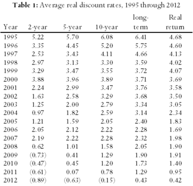
In Table 1, we summarise those rates for five-year, ten-year, long-term, and real rate of return bonds and for GICs of one-year, three-year, and five-year terms. In this table, the term “long-term bond” applies to government bonds with maturation dates of fifteen years or more. “Real rate of return bonds” are bonds whose rate of return is specified as a fixed value (the real rate of return) plus the actual rate of inflation. Thus, for example, if the fixed value is 1.0 percent and the rate of inflation proves to be 2.5 percent, the bond will pay (approximately) 3.5 percent.²

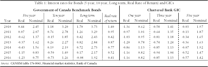
Table 1 reports both the nominal (observed) and real (net of inflation) rates of return on five- and ten-year bonds, long-term bonds, and GICs. In each case, the real rate has been calculated by reducing the nominal rate by the expected rate of inflation, two percent.³ As the interest rate on real rate of return bonds is reported as a real rate, we report only the real rate of return on those bonds.

In Table 1 it can be seen, first, that the real rates of return on government bonds increase as the duration of those bonds increase; thus confirming that there is not a single discount rate but rather a different rate for each length of investment.

Second, it is also seen that the real interest rates on secure bonds have not recently risen above 0.5 percent for investments of any duration; and have risen above 0.0 percent only on real rate of return bonds.

Our contention is that these rates can be used as indicators of the rates at which life insurance companies will invest the funds they receive for life annuities and structured settlements. We can test this contention by comparing the interest rates employed to determine the prices of structured settlements against the rates reported in Table 1.

This we have done by obtaining quotes for several alternative structured settlements. From these we have been able to determine the interest rates that were employed to obtain those quotes. In Table 2 we report six such structured settlements, for males receiving $1,000 per month ($12,000 per year).⁴

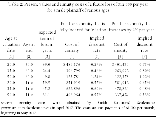
Three scenarios represent payments that end at age 60 and three represent payments that continue to the date of the plaintiff’s death. (Those that end at age 60 are assumed to be typical of awards for loss of earnings; and those that continue for life are assumed to be typical of awards for medical expenses.) The assumed ages for the plaintiffs, at the date of trial, are, respectively, 20, 35, and 60. Furthermore, in each case we report quotes for both the situation in which the annual payment is to increase by two percent per year and for that in which it will increase by the actual rate of inflation.

Column (4) of Table 2 reports the quotes we received, assuming that the annual payment was to increase by the actual rate of inflation; while column (6) reports the quotes assuming that the annual payment was to increase by two percent per year. Columns (5) and (7) then report our calculation of the implied interest rates that were used to obtain the costs of the various annuities.

For example, the first figure in column (4) indicates that it would cost $489,176 to purchase an annuity that paid a male plaintiff $12,000 per year, indexed for inflation, for the next 40 years (i.e. from age 20 to age 60). The first figure in column (5) then indicates that the insurance company that quoted this amount had implicitly assumed that its investments would earn an average real rate of interest, (i.e. nominal interest net of inflation), of -0.27 percent over the 40-year period in question. Similar costs and real interest rates are reported for the other eleven scenarios.

Notably, in every case in which the payments were fully indexed for future inflation (column 5), the implied real rate of interest was negative – between -1.24 percent and -0.27 percent. It is only when the payments did not provide full protection against inflation – column 7, in which increases were limited to two percent per year – that insurers offered a positive real interest rate. Even then, rates were less than one percent.

We would note that the implied discount rates of the annuities presented in Table 2 are consistent with the implied discount rates of annuities offered by private insurance firms such as Sun Life Financial and RBC Insurance. For example, the Sun Life Financial annuity calculator indicates that as of April 2017, a $1,000,000 annuity for a 50-year old female will provide an annual income of approximately $41,819 per year (with no inflation adjustment). This implies a discount rate of approximately 0.13 percent. The annuity calculator provided by RBC Insurance indicates that as of April 2017, a $1,000,000 annuity will provide a 55-year old male with annual payments of approximately $50,931 (with no inflation adjustment), for an implied discount rate of 0.15 percent.⁵

It is informative to compare the rates employed in the calculation of structured settlements (and private annuities) with the rates reported for government bonds, in Table 1. The two annuities with the shortest durations – ten years, from age 50 to 60 – had implied discount rates of -1.24 and -1.02 percent, both very similar to the figure of -1.23 percent reported in Table 1 for five-year bonds in 2016. Similarly, the two annuities with the longest durations – from age 20 for life – had implied discount rates of -0.57 percent and +0.65 percent, with an average very close to the figure of -0.08 percent reported in Table 1 for long-term government bonds.

We conclude from Tables 1 and 2 that, in cases in which the plaintiff purchases a life annuity or structured settlement – particularly one that is fully indexed for inflation – the discount rate can be estimated with some accuracy from the real rates of return currently available on Government of Canada bonds of appropriate durations.

2. Active Management Approach

In the active management approach, it is assumed that plaintiffs will re-allocate funds within their investment portfolios as conditions in financial markets change. Because these changes will be made in the future, the active management approach requires that estimates of future rates of return be calculated.

In this section, we first identify the type of financial instrument in which we assume the plaintiff will invest. We then contrast two methods of forecasting the rates of return on those instruments. Finally, we provide estimates of those rates of return.

Selection of the Appropriate Financial Instrument

The courts have been clear that, as the lump-sum award is intended to replace the plaintiff’s lost earnings, the investments in the plaintiff’s portfolio must not expose the plaintiff to unreasonable risk. For example, in its seminal decision in Lewis v. Todd (1980 CarswellOnt 617), the Supreme Court of Canada approved of the expert’s use of “high grade investments [of] long duration” [para. 17].

As the rates of return on investments in the stock market have historically been very volatile, it is usually recommended that plaintiffs do not restrict their investments to equities. Table 3, for example, reports the value of the Toronto Stock Exchange composite index for July of each year since 2000. It can be seen there that rates of return have been highly volatile, indicating that the rate available to an individual whose investments tracked the market would have depended importantly on the year in which those investments were made. For example, whereas the nominal return on investment in such a portfolio would have averaged 2.2 percent per year between 2000 and 2015, a similar investment would have averaged 6.2 percent per year between 2002 and 2015.

In light of this issue, two approaches might meet the court’s requirement that plaintiffs invest in high grade investments: it could be assumed that plaintiffs will purchase long-term Government of Canada bonds; or that they will invest their awards in financial instruments that offer higher yields than government bonds, but with greater risk – for example, in a mixed portfolio of “blue chip” stocks, corporate bonds, and mutual funds. In the discussion that follows, we will consider both.

Forecasting the Returns on Government Bonds

Two methods have commonly been used to forecast the rate of interest that will be available on government bonds. The first of these, the historical approach assumes that future rates will equal those that were observed in the past. The second, the efficient market approach, assumes that the rates that are currently available in the market reflect the rates that investors believe will prevail in the long run. We explain here why we prefer the efficient market approach.

The historical approach: A fundamental problem with the historical approach is that real interest rates have varied significantly over the last sixty years. As can be seen from Table 4, real rates were as low as 1.50 percent in two decades (1951-1960 and 1971-1980) and as high as 4.70 percent in two others (1981-2000). From this record, it would be possible to find support for almost any long-run rate between 2.0 and 5.0 percent.

More importantly, as indicated in Figure 1, real rates of return have declined virtually continuously for the past twenty years, from approximately 5.5 percent to -0.5 percent. Even if it was to be argued that real rates of interest will return to, say, 3.0 percent over the next twenty years, most plaintiffs will experience rates of return well below that over most of the period in which their award is invested.

A third problem with the use of historical rates is that there is no theory to support it. Adherents simply assume that because real rates took some value in the past, rates will return to that value in the future. Furthermore, they make this assumption in the face of the long run decline in real interest rates reported in Figure 1. If the markets expected the real rate of interest to return to “long-run” levels soon, sophisticated investors would not continue to purchase financial instruments that paid long-run rates as low as -0.08 percent (Table 1).

Finally, the evidence is not just that the real interest rate has declined significantly; this decline is consistent with theoretical predictions. Importantly, as central banks have adopted a policy of maintaining inflation within a narrow band of rates (in Canada, between 1.0 and 3.0 percent), uncertainty about the rate of inflation has been minimized. This reduction in risk has led to an increase in demand for bonds, and an associated reduction in real interest rates.

The Congressional Budget Office of the United States also predicts that interest rates will be lower in the future than in the past, resulting in part from slower growth rates of both the labour force and of productivity, thereby reducing the rate of return on capital; and in part from a shift of income to high-income households who tend to have high savings, thereby increasing the supply of money to the bond market.

The efficient market approach: The second source of information concerning future real rates of interest is the money market. When an investment firm that believes that inflation will average two percent per year purchases twenty-year Government of Canada bonds paying three percent, it is revealing that it expects the real rate of interest on those bonds will average approximately one percent over those twenty years. Thus, if the rate of inflation that investors were forecasting was known, that forecast could be used to deflate the nominal rates of interest observed in the market to obtain the implicit, underlying forecasts of real rates.

A strong case can be made for using an expected inflation rate of two percent. The reason for this is that in the last decade the Bank of Canada has not only made this its target rate of inflation, it has been successful in keeping the actual (long-run) rate of inflation very close to that target (which, in turn, has led most financial institutions to predict that future inflation will average two percent).⁶

Furthermore, in choosing to target a low rate of inflation, the Bank has been following a view that has achieved widespread acceptance in the economics community – that is, that control of inflation, at a low level, should be one of central banks’ primary roles.

On this basis, at the end of 2016 the real rate of interest on long-term government of Canada bonds appeared to be as little as 0.00 percent. (See the figures for long-term bond rates in Table 1.)

An alternative approach is to rely on information concerning bonds whose rate of return is denominated in terms of real interest rates – called real return bonds, or RRBs. By observing the rates of return at which these bonds sell, the risk free real rate of return that investors believe will prevail over the long run can easily be determined. That is, even if plaintiffs do not purchase RRBs, the real rate of interest that is observed on those bonds provides an unbiased indicator of the rate of interest that is expected by sophisticated investors. In Table 1, it is seen that the return on these bonds has recently fallen to as little as 0.41 percent.⁷

Forecasting Returns on a Mixed Portfolio

Forecasting the returns on a conservative, mixed portfolio is complicated by the fact that there is no common agreement about what the components of such a portfolio should be. Hence, not only is it difficult to obtain the current rates of return on conservative investments, there is also very little information about how such returns have varied over the past. Both issues complicate the forecasting process.

An approach that we suggest might mitigate this problem would be to rely on the rates of return that have been available on conservative portfolios offered by Canadian banks. We have been able to obtain information about four of these: the RBC Select Very Conservative Portfolio, CIBC Managed Income Portfolio, TD Comfort Conservative Income Portfolio, and ScotiaBank Selected Income Portfolio-Series A. Although these funds differ from one another in their details, they all have investment objectives similar to those stated for the RBC portfolio:

To provide income and the potential for modest capital growth by investing primarily in funds managed by RBC Global Asset Management, emphasizing mutual funds that invest in fixed-income securities with some exposure to mutual funds that invest in equity securities. The portfolio invests in a mix of Canadian, U.S. and international funds.

To achieve this goal, RBC invests primarily in bond funds. The result, seen in the first columns of Table 5 below, is that since 2011 this fund has consistently earned a nominal rate of return between 2.5 and 5.0 percent – with one deviation, to 6.74 percent, in 2014 – suggesting a real rate of return over that period of approximately 1.0 to 3.5 percent. Table 5 reports similar results for the other three portfolios (again, with 2014 being the only year that each of them achieved a nominal return that exceeded 5.00 percent).

The volatility in the rates of return on all four portfolios reported in Table 5 is considerably less than that on investments in the Toronto Stock Exchange, as reported in Table 3.

But that does not necessarily mean that plaintiffs would be advised to invest in a conservative mixed portfolio. Although the returns on such portfolios may be higher than that on life annuities, the returns on the latter are fixed once they are purchased, and hence have lower (zero) volatility than the returns on all other investments. The question remains: do the higher rates of return on mixed portfolios compensate the plaintiff for the higher volatility of their returns? This is a question that cannot be answered by financial experts, but only by the courts or government regulators.

What Table 5 does suggest, however, is that if plaintiffs had purchased mixed conservative portfolios in the last five years they would have achieved average nominal returns of between 3.5 and 4.5 percent per annum – or approximately 2.0 to 3.0 percent in real terms. This suggests that 2.5 percent represents a conservative estimate of the real rate available to plaintiffs seeking conservative investments.

III. Summary

In personal injury and fatal accident actions, the plaintiffs are assumed to invest their awards in such a way as to provide streams of returns that will replace their future annual losses. Two factors may intervene to hinder plaintiffs’ ability to achieve this goal. First, they may live longer than average. Second, the rate of return on investments may fall below the level that was anticipated when calculating their awards. In both cases, the award will be exhausted before the plaintiff’s death.

One approach plaintiffs can employ to avoid these problems is to invest their awards in life annuities or structured settlements, as these instruments guarantee a specified annual payment for life, and as the rates of return available on them are fixed.

The drawback to annuities is that the interest rates that insurance companies use to price their products are much lower than the rates of return that have been available on conservative mixed portfolios of financial assets. We showed in Section II that, whereas the implicit interest rates on life annuities are similar to the rates available on long-term Government of Canada bonds, or approximately 0.0 to 0.5 percent, the interest rates available on conservative portfolios of assets have been approximately 2.0 to 3.0 percent.

If a loss will not continue into the years beyond which mortality rates begin to rise substantially, the advantage of buying a life annuity may be relatively small compared to investing in a portfolio of assets. In that case, it may be appropriate to assume that that the discount rate can be estimated from the return on a portfolio of assets.

If the loss will continue into years of high mortality, however, the benefits of a life annuity (protection against exhaustion of the award) may exceed the costs (a lower rate of interest).

As it is only the plaintiff who can determine whether the benefits of a life annuity exceed the costs, it seems appropriate that the discount rate be chosen based on the plaintiff’s decision whether to self-manage the investment of his or her award or to use that award to purchase a life annuity (or structured settlement).

If the plaintiff chooses to self-manage his or her award, we recommend that the discount rate be set at 2.5 percent.
If the plaintiff chooses a life annuity or structured settlement, we recommend that the discount rate be set at zero percent.
We anticipate that plaintiffs will make the latter choice in virtually all cases in which their losses will continue into years of high mortality.

The Structure of a Cost of Care Report

Posted on June 1, 2016March 26, 2017 By economica

by Christopher J. Bruce, Kelly A. Rathje

As economists, we are often asked to calculate the present value of future costs of care. As these calculations are based on the reports of cost of care experts (CCEs), we have become uniquely familiar with the structure and content of those reports.

In this article, we provide a review of the format and contents of cost of care reports, drawn from our experience using those reports as inputs into our own calculations. We anticipate that this review will be of greatest use to:

members of the bar: as a checklist against which to evaluate the cost of care reports that have been provided for them and their opponents;
individuals who have recently begun preparing cost of care reports: to provide them with an understanding of how those reports will be used; and
experienced cost of care experts: as an analysis of some of the complexities that can arise in personal injury actions. For these experts, most of our suggestions will be familiar; but we hope that we raise sufficient questions to make this report of interest to them also.

Incremental Costs

One of the most difficult questions facing the cost of care expert (CCE) is that of distinguishing between those costs that would have arisen had the plaintiff not been injured and those that have arisen as a result of the plaintiff’s injuries. This issue is particularly important when the item required with-accident differs only in quality or type from a similar item that would have been purchased without-accident, for example when the plaintiff now requires a different type of automobile than she would have purchased had she not been injured.

A number of issues arise with respect to incremental costs:

1) When the item required by the plaintiff costs more than the equivalent item for a non-injured person, it is important to be very clear about what is being assumed about the characteristics of the item that would have been purchased by the non-injured person. For example, assume that it has been recommended that a paraplegic purchase a van that costs $45,000 per year. As the incremental cost is the difference between that $45,000 and the cost of the car the plaintiff would have purchased if he had not been injured, it is important that the CCE be able to defend any assumption that has been made about the cost of the latter. Would the plaintiff have owned a Honda that cost $20,000, or a Lexis that cost $50,000? On what basis has that conclusion been reached?

2) Following from the preceding point, it is also important to alert the reader to the possibility that the item that has been recommended by the CCE may be of a different quality than the item the plaintiff would have purchased had she not been injured. Would a $45,000 van, for example, “replace” a $50,000 Lexis? And would the quality of accommodation and food in, say, a nursing home replace the equivalent items in the plaintiff’s own home?

3) An important example of quality differentials arises with respect to the care of injured children. Assume that a child’s injuries are sufficiently severe that the CCE has recommended that professional child care be provided for her – for example, 24-hour attendants. Assume also that the child has a stay-at-home mother; that is, one who would have provided 24-hour care before the child began school. Can it be argued that, as the child would have received 24-hour care in the absence of the accident, the accident has not caused any increment in costs? The answer to this question depends on whether the type and extent of care (i.e. the “quality” of care) that the child now needs exceeds that which would normally have been provided by her parents. For example, during the ten hours that the child normally sleeps, incremental care might be recommended because she will wake more often than normal, or because specialized medical care will be required during those hours. If so, it would be useful if this was specified in the cost of care report. Similar specifications may also be necessary with respect to time that a non-injured child would have spent at school or in day-care.

4) When estimating what the plaintiff would have spent on a category of items if he had not been injured, a distinction must be made between the expenditures that he is currently incurring and those that he would have incurred if he had not been injured. For example, if the accident has reduced the plaintiff’s income, it is quite possible that he will now be living in an apartment with a lower monthly rent than he would have incurred had he not been injured. It is the difference between the rent of the apartment the CCE has recommended (with-accident) and the rent of the apartment he would have lived in (without-accident) that is the incremental cost due to the accident.

5) If the item owned by an injured plaintiff has a longer or shorter life expectancy than the equivalent item owned by a non-injured person, the CCE should identify what that difference is. For example, the van required for a paraplegic might have a five-year use life, whereas the car that the plaintiff would have driven if she had not been injured might have had a ten-year life. In such a case, it would not be appropriate to calculate the incremental cost by deducting the purchase price of the car the plaintiff would have bought from the purchase price of the van, as two vans will have to be purchased for each car.

Variations over Time

The requirements for many items will vary over the plaintiff’s lifetime. It is important to identify when such changes will occur and what their effect will be on annual costs:

1) The plaintiff would have incurred some of the costs of care at various times in his lifetime even if he had not been injured. For example, at age 80, the plaintiff may have hired a housekeeper. Thus, if the CCE had recommended housekeeping services from the date of the accident, for life, the cost that would have been incurred after 80 must be deducted from the recommended expense. In such cases, it would be useful if the CCE was to indicate the age at which the plaintiff would have incurred the stated expense (in the absence of the accident), and what the difference is between the cost of the recommended level of housekeeping and the level that would have been purchased had the accident not occurred.

2) It is important to be clear about variations in expenses over the course of a year – such as due to school holidays and vacations – and over a lifetime – such as because the plaintiff would have started elementary school, entered university, had children, or retired.

3) If the plaintiff will have to undergo surgery in the future, the CCE should indicate how long the recovery period will be and how much the extra costs will be during that period. Also, it will be useful to the economist to know whether the plaintiff will be able to return to work before the end of the recovery period.

Ranges of Estimates

We often find that CCEs provide a range of estimates for the cost of a recommended item. For example, it might be reported that the cost of personal care attendants will vary from $14,500 per year to $21,400. When the CCE wishes to report such a range, we recommend that a reason be provided why a single number would not be appropriate, and the source was of each of the costs in the range be identified. For example, if there is more than one cost, that might be because:

the CCE received more than one quote, from more than one provider (and if so, why was the lowest quote not chosen?);
there were different costs for different qualities of the product;
different costs were appropriate to different potential medical outcomes;
costs varied among cities in which the plaintiff might live; etc.

Housekeepers and Personal Care Attendants

The CCE report should clearly specify the sources for the hourly costs of individuals who provide housekeeping services, such as housecleaners, yard workers, and maintenance workers. Otherwise the cost of care report may be subject to criticism from experts, such as economists, who are familiar with data concerning the wage rates of these individuals.

Once it has been determined how many hours are required for each type of personal care attendant (for example, nurses and LPNs), there are two basic approaches to estimating the cost of those individuals. The first of these, the agency approach, is to obtain the cost of hiring an agency that will be responsible for all of the specified activities. The second, the hourly wage approach, is to obtain an hourly wage for each type of attendant and then multiply those wages by the specified hours for each type.

Although the latter approach often appears attractive, in the sense that it yields a lower estimate of costs than does the former, there are many reasons to be cautious about use of this approach. First, unless the plaintiff is capable of handling his/her own affairs, the hourly wage approach often assumes that there is a family member who will work without compensation to hire and supervise attendants. But, even if such individuals are available currently, there is no assurance they will be available over the entire course of the plaintiff’s disability. Furthermore, in those years in which family members are available to assist the plaintiff, the courts will generally allow them to claim for the costs of their time, invalidating the assumption that their time is “free”.

Second, the hourly wage approach may not take into account that substitutes will have to be provided for attendants who are ill, wish to take vacations, or who quit without warning.

Third, allowance has to be made for the possibility that attendants will not provide adequate care. This requires that the family or plaintiff have some expertise in both the investigation of the backgrounds of potential hires and in the provision of supervision of existing employees.

Finally, the hourly wage approach would have to provide an allowance for the hiring of additional personnel when emergencies arose. Whereas most agencies will be able to call on their own nurses, and will have close contacts with doctors, ambulances, and hospitals; the plaintiff and his/her family will generally have no expertise in hiring these experts.

Other Factors

We also make the following recommendations concerning the cost of care report:

1) The report should indicate whether GST is included or excluded in the costs recommended.

2) As some items will be GST-exempt while others will not, it is important to distinguish between the two.

3) Indicate whether the costs identified for a particular item are for a different year than the one in which the report was written. For example, if a report was written in 2015, the costs may have been collected from 2014 price lists, or may have been forecasted for a settlement date in 2016. [We generally assume that a report written in 2015 uses “2015 prices”.]

4) It may be advisable, particularly in contentious cases, to have a physician read the CCE’s report and approve the medical expenses, in writing.

Presentation

In addition to the recommendations we have made above, concerning the content of the cost of care report, we also have a number of (minor) suggestions concerning the format, or presentation, of that report:

1) We appreciate it when the CCE provides a summary table in which the annual cost of each item is clearly set out, along with the number of years each cost is to be repeated. We acknowledge that at times, a unit cost, such as medication costs per unit, plus the number of units required over a specific time period is provided. This is just as useful to us, as from this information we can easily determine an annual cost¹.

2) If an expenditure is to be made less often than annually – for example, replacement of a car or wheelchair once every five years – it is not necessary for our purposes that the CCE averages the costs over the life of the item. Provide only the replacement cost and the number of years between replacements.

3) On items like cars, houses, and wheelchairs, the cost of care report should, however, provide the annual costs of repair, maintenance, and operation. For a car, for example, provide estimated costs of repairs, of oil changes, and gasoline and tires.

4) The report should be clear about time ranges. For example, it is confusing to say that an item will cost $600 per year from age 25 to 35 and $450 from age 35 to 45, as that leaves it unclear what the cost will be at age 35. We would recommend, instead, that the report say something like: the item will cost $600 per year from 25 to 35 and $450 per year from 36 to 45.

5) There is no need to “round” numbers up or down as economists use spreadsheets for their calculations.

A Sample Economist’s Report

As the economist’s report is always written after the cost of care expert’s report, we suspect that many CCEs will not have seen very many economist reports. As it may help the CCE to understand what types of information are required for an economist report, and in what format that information should be provided, in the table presented below we provide a sample copy of a cost of care calculation for a hypothetical seven-year old male plaintiff.

In the footnote to the table, we have also provided an example of a typical assumption we would make when a range of replacement times has been provided by the CCE.

The columns in the table have the following interpretations:

Tax creditable expense: “Y” in this column indicates that the item can be claimed as a medical expense for income tax purposes.

Cost including tax: the cost of the item, including all taxes.

Replacement life: This column reports the frequency of expenditure. “0” in this column means that the item is purchased only once (there is no frequency); “1” means that the item is purchased every year; “2” means that it is purchase once every two years, etc. For example, under “Mobility” the “Ankle/foot orthotic (adult)” is to be replaced once every three years; the “Adapted bike,” however, is to be purchased only twice, at ages seven and fourteen.

Starting age: The age at which the item is first to be purchased. As the hypothetical plaintiff is seven years old, most purchases begin at seven. However, it is seen, for example, that many items in this table are not to be incurred until the plaintiff is eighteen.

Ending age: Many of the items are to be purchased only over a portion of the plaintiff’s life. Often, as in this case, the costs are different when the plaintiff is a child than when he/she is an adult, and costs may change again when the plaintiff retires or enters a senior’s facility.

Present value of costs: This is the lump sum that would have to be invested today to provide the plaintiff with sufficient funds to replace the stream of future costs in each row. For example, a “Before/after school, weekend care” expenditure of $56,060.76 per year from age seven to thirteen will cost $309,468. This figure varies according to the annual cost, the duration of the expenditure, the discount rate, and the plaintiff’s life expectancy.

Multiplier: Assume that the cost of care expert has recommended an expenditure of $1,000 per year for the next ten years, and that the present (lump-sum) value of this cost has been calculated to be $8,300. If that expenditure was to be doubled, to $2,000 per year over the same time span, the present value of the cost would also double, to $16,600. Alternatively, we can represent this by saying that for every $1.00 of annual costs (over this ten-year span), the present value of future costs will be $8.30. Any lump-sum cost can be obtained by multiplying the annual cost by 8.30. The latter figure is called the “multiplier.” It can be used by the court to recalculate the present value of future costs if the court should conclude that the annual costs are different from those recommended by the cost of care expert.

For example, if the court was to rule that annual before/after school costs were $40,000 (instead of the $56,060.76 reported in the table, the present value would be $40,000 multiplied by the reported multiplier, 5.52, yielding $220,800. [Note: there is a separate multiplier for each starting/ending age combination. Multipliers also differ if a different discount rate or life expectancy is used.]

Sample Cost of Care Calculation for Seven-year-old Plaintiff

* The cost of care expert recommended that the wheelchair be replaced approximately every three to five years. It was also indicated that once the child’s chair had reached its maximum capacity, it would have to be replaced with an adult chair. For the purposes of our calculations, we have assumed that the chair will require replacement every four years until the plaintiff is eighteen.

We would like to thank Stephen Kuyltjes of Rehab Works, Calgary; Sharon Kaczkowski of Kaczkowski Occupational Therapy, Calgary; and Everett Dillman of International Business Planners, El Paso, Texas, all of whom were kind enough to comment on earlier drafts of this article. We are responsible for any remaining errors or omissions.

Christopher Bruce is the President of Economica and a Professor of Economics at the University of Calgary. He is also the author of Assessment of Personal Injury Damages (Butterworths, 2004).

Kelly Rathje is a consultant with Economica and has a Master of Arts degree (in economics) from the University of Calgary.

The Effect of Incarceration on Future Earnings

Posted on June 1, 2016March 26, 2017 By economica

by Christopher J. Bruce, Derek W. Aldridge

In personal injury and fatal accident claims, the courts are often required to determine what effect a criminal record would have had on the earnings of the plaintiff. We suspect that most individuals would expect that criminals will have lower wages and higher unemployment rates than the average citizen.

In this paper, we summarise the most reliable research that has been conducted into this question. We divide this summary into four lines of investigation: the impact of incarceration on earnings and employment; the effect of an increase in the duration of incarceration; the determinants of a successful transition from jail to civilian life; and the determinants of the probability of recidivism.

Incarceration

Although the raw data indicate that those who have been incarcerated have lower earnings and higher unemployment rates than those who have no criminal record, research indicates that this is an example of “correlation, not causation.” (For further information on the misuse of statistics in legal proceedings, see Bruce, 2004.) That is, careful analysis of the data have shown that individuals with low earnings and high unemployment rates are more likely to commit (and be convicted of committing) crimes than are those with high earnings and low unemployment rates. Hence, the primary reason that earnings are low among those who have been incarcerated is that those individuals are drawn from a population of individuals who have low earnings, not because the incarceration changed their employment prospects.

Grogger (1995), for example, found that neither arrests nor jail terms had long term effects on the earnings or employment of young men. And Kling (1999) concluded that, for most individuals, incarceration only reduced earnings by 0 to 3 percent, five to eight years after release. The only group for whom incarceration had a significant effect on post-release earnings was white collar criminals (such as accountants and stockbrokers). Similarly, Richey (2015) found that the effect of conviction on earnings was small or zero. Western (2002), however, found that although conviction had no effect on employability, it reduced the rate of growth of earnings by approximately 33 percent. (Note, however, that as rates of growth are often approximately two or three percent per year, a 33 percent reduction implies a reduction in rate of growth of approximately one percent or less.)

Duration of incarceration

A number of recent articles have attempted to determine whether an increase in the length of a jail sentence, holding the severity of the crime constant, has an effect on post-incarceration employment and earnings. One study found that there “…. is no substantial evidence of a negative effect of incarceration length on employment or earnings.” (Kling, 2006) Another found that the length of prison sentence for drug offences had no significant effect on earnings; but that length of sentence had a very significant effect with respect to incarceration for fraud and embezzlement. (Lott, 1992)

Transition from prison into the workplace

A small number of studies have investigated the factors that influence the success of transition out of prison. Typical of these is Visher and Travis (2003) in which the authors found that men with close ties to families and friends made the most successful transitions into the workplace, particularly if they lived with their wives and children. Families appeared to be especially important if they provided emotional support and housing assistance.

Recidivism

Numerous studies – e.g. Gendreau et. al. (1996), Jones (2005), and Motiuk and Vuong (2005) – have concluded that those who have been released from prison are more likely to reoffend if they have experienced high levels of unemployment or job instability, lack a skill or trade, or are drug users. They are also more likely to reoffend the younger they are.

The finding that it is younger individuals who are most likely to re-offend implies that most offenders have left the criminal population by the time they are in their late 20s. One Canadian study (Correctional Service of Canada, 1993), found that, at age 32, the average age at which respondents had committed their last offence was 23. A subsequent study (Ouimet and LeBlanc, 1996), based on interviews with 238 young men who had previously been young offenders, found that whereas more than half had been criminally active between the ages of 18 to 25, only 18 percent had been criminally active after 25.

Summary

The scientific literature suggests that incarceration has a relatively small effect on lifetime earnings. Although those who have been incarcerated earn lower incomes than those who have not been incarcerated, it is primarily because they are drawn from a group that tends to have relatively low earnings, not because the incarceration “causes” low earnings. Further, the data appear to indicate that the likelihood of being convicted and sent to jail decreases as an individual ages. Hence, those 30 and 40 year olds who were incarcerated in their early 20s are not likely to become repeat offenders.

It appears, therefore, that once a plaintiff reaches the age of approximately 25, the best predictors of his future earnings are standard factors like earnings history, education, and occupation. Whether or not that individual has been incarcerated will not add a significant amount of information to the factors that are used to forecast earnings of non-incarcerated individuals.

Sources

Bruce, Christopher, (2004) “The Reliability of Statistical Evidence Concerning the Impact of Disability;” Expert Witness, 9(4), http://www.economica.ca/ew09_4p1.htm.
Correctional Service of Canada, (1993) “Recidivists tend to be…;” Forum on Corrections Research, 5(3).
Gentreau, P. et. al. (1979) “Norms and recidivism for first incarcerates: Implications for programming;” Canadian Journal of Criminology, 1-26.
Grogger, J. (1995) “The effect of arrests on the employment and earnings of young men;” Quarterly Journal of Economics, 51-71.
Jones, D. (2005) “Offender employment: A research summary;” Forum on Corrections Research, 17(1), 13-20.
Kling, J. (1999) “The effect of prison sentence length on the subsequent employment and earnings of criminal defendants;” Woodrow Wilson School Discussion Papers in Economics.
Kling, J (2006) “Incarceration length, employment, and earnings;” American Economic Review, 863-876.
Lott, J (1992) “Do we punish high income criminals too heavily?;” Economic Inquiry, 583-608.
Motiuk, L, and B. Vuong (2005), “Offender employment: What the research tells us;” Forum on Corrections Research, 17(1), 21-24.
Ouimet, M., and M. LeBlanc (1996) “Life events in the course of the adult criminal career;” Criminal Behavior and Mental Health, 6(1), 75-97.
Richey, J. (2015) “Shackled labor markets: Bounding the causal effects of criminal convictions in the U.S.;” International Review of Law and Economics, 41, 17-24.
Visher, C., and J. Travis (2003) “Transitions from prison to community: Understanding individual pathways;” Annual Review of Sociology, 29, 89-113.
Western, B. (2002) “The impact of incarceration on wage mobility and inequality;” American Sociological Association, 4, 526-546.

Christopher Bruce is the President of Economica and a Professor of Economics at the University of Calgary.

Derek Aldridge is a consultant with Economica and has a Master of Arts degree (in economics) from the University of Victoria.

Are Data from the 2011 Census Reliable?

Posted on March 1, 2016April 18, 2017 By economica

When estimating future earnings in personal injury and fatal accident cases, financial experts often rely on information provided by the Canadian Census. Of particular importance are data concerning incomes by age, sex, occupation, and education. For example, if a 24 year-old male plaintiff would have been a journeyman carpenter, his potential earnings might be based on average incomes for Canadians with that certification, in the age groups 25-29, 30-34, 35-44, etc.

In the past, these data would have been drawn from a section of the Census known as the “long form.” This portion of the Census survey, which contained much more detailed information than on was on the rest of the Census, was given to only one household out of five. (The remainder of the Census survey asks only basic questions about such demographic factors as age, sex, language, and area of residence.)

For the 2011 Census, however, the government decided to replace the long-form questions with a “National Household Survey (NHS).” Although the 2011 NHS asked the same questions as had the 2006 Census long form, whereas the long form had been mandatory, the NHS was voluntary. The result, as had been expected, was that the percentage of households answering this portion of the survey fell significantly, from 93.8% in 2006 to 77.2% in 2011.This created three statistical problems concerning the reliability of the data (variability in small community data, sample error, and non-response bias). As Statistics Canada had anticipated these problems, however, it took steps to mitigate them, steps that have maintained the reliability of the data that are of value to the courts. Wayne R. Smith, Chief Statistician of Canada, recently wrote an article in which he discussed these steps. [“The 2011 National Household Survey – the complete statistical story,” http://www.statcan.gc.ca/eng/blog-blogue/cs-sc/2011NHSstory. June 4, 2015.] In this article, I summarise Dr. Smith’s discussion.

Variability in small community data

As the sample size of any survey becomes smaller, the data become less and less reliable, due to an increase in variance. In response, Statistics Canada routinely withholds data concerning the smallest communities. In 2011, they withheld the results from 1,100 such communities, up from 160 in the 2006 Census. That is, all of the data reported in 2011 meet the normal statistical requirements for reliability.

Sample error

As the overall size of a sample decreases, there is an increase in what is known as the “sampling error;” that is, from the problem that the average characteristics of the sample differ from the average of the total population. Because Statistics Canada expected a smaller percentage of households to answer the voluntary NHS than had answered the mandatory long form, they anticipated that the total size of the “sample” (the households answering the survey) would be lower in 2011 than in 2006.

To deal with this problem, Statistics Canada increased the number of households who were asked to answer the long portion of the 2011 Census. Whereas one household in five were asked to answer the 2006 long form, one household in three were asked to answer the NHS. The result was that, even though a smaller percentage of households responded to the NHS than had responded to the 2006 long form, the number of households answering the NHS was higher than in 2006, (2,657,461 versus 2,443,507, representing 6,719,688 versus 2006’s 6,136,517).

Although this approach does not correct for all errors, those errors become less and less important as the data are aggregated. Thus, for example, the data for the average income of all carpenters in Alberta are more reliable than for the average income of carpenters in Calgary.

Non-response bias

The most worrisome problem that arises when a survey is made voluntary is that the households who choose to respond to that survey may differ significantly from those who refuse to do so. For example, if those carpenters with relatively high incomes are more likely to respond to the NHS than are those with low incomes, the average incomes reported by the NHS will be biased upwards.

Statistics Canada could not control, ex ante, for the possibility that this would happen. However, they were able, ex post, to investigate whether the respondents to the NHS were representative of the overall groups from which they were drawn – that is, they were able to determine whether the respondents “looked” different from the average.

To make this determination, Statistics Canada was assisted by the fact that they had a considerable amount of information about the respondents to the NHS before those individuals answered the NHS survey. Most importantly, they also had their responses to the short questions on the Census that are mandatory for all Canadians. In addition, they were also able to link the NHS respondents to those individuals’ tax files, immigrant landing data, and the Indian Register.

Using sophisticated statistical techniques they were able to determine that the average respondent to the NHS had very similar characteristics to the average Canadian with respect to age, sex, language, area of residence, income tax, immigration status, and aboriginal status. This finding leads Statistics Canada to conclude that the NHS respondents were, in most cases, representative of the larger population from which they were drawn. And when Statistics Canada was unable to conclude that the individuals who replied to a specific sub-class of questions were representative of the population, the resulting data were not released, or they were released with an accompanying cautionary note.

Summary

To summarise: Although the long-form portion of the 2011 Census was made voluntary, there is sound reason to believe that the data that are of greatest relevance to the calculation of lost earnings can be relied upon.

The information in this article is drawn from a blog written by Wayne R. Smith, Chief Statistician of Canada, entitled “The 2011 National Household Survey – the complete statistical story,” June 4, 2015. This blog can be found at: http://www.statcan.gc.ca/eng/blog-blogue/cs-sc/2011NHSstory.

Christopher Bruce is the President of Economica and a Professor of Economics at the University of Calgary. He is also the author of Assessment of Personal Injury Damages (Butterworths, 2004).

Cross versus Sole Dependency in Fatal Accident Actions

Posted on March 1, 2016March 26, 2017 By economica

[back to text of article]

When a spouse has been killed through the negligence of a third party, the surviving spouse is entitled to damages that would allow him/her to maintain the standard of living that he/she had previously enjoyed.

The determination of this value requires that three steps be taken. First, the potential earning capacity of each spouse must be estimated. Second, a calculation must be made of each spouse’s dependency rate – that is, the percentage of family income that benefitted that spouse. Third, it must be determined whether any monies that had been spent on the deceased by the survivor (and which now do not have to be spent due to the death of the former) should be deducted from the survivor’s loss of dependency. In what is known as the sole dependency approach, that “saving” is not deducted. In the cross dependency approach, the saving is deducted.

In this article, I will use a concept that is fundamental to economic analysis – the rational person assumption – to suggest that basic economic principles favour the use of sole dependency.

I begin by making some simple assumptions about a couples’ earning capacity and dependency rates and use those assumptions to define sole and cross dependency. I then introduce the rational person assumption and provide examples of the use of that assumption in non-fatal accident cases. Finally, I extend the analysis to fatal accident cases and argue the rational person assumption provides support for use of the sole dependency approach.

Assumptions concerning earning capacity and dependency

Statistical analyses suggest that, in a household consisting of a husband and wife, approximately 30 percent of the family’s after-tax income is spent on items such as food, clothing, and transportation that benefit the husband alone; approximately 30 percent is spent on items that benefit the wife alone; and 40 percent is spent on items, such as housing, furniture, and insurance, that benefit both spouses collectively. Each spouse benefits, in total, from 70 percent of family income – 30 percent that benefits that spouse personally – usually referred to as “personal expenses” – and 40 percent that benefits both spouses equally – “common expenses.” The 70 percent figure in this example is known as the individual spouse’s “dependency rate.” [Note that, as both spouses have the same dependency rate, 70 percent, there is a net benefit from marriage.]

Assume that in a childless couple, the husband earns $100,000 per year after taxes and the wife earns $40,000. Based on my assumptions concerning dependency rates, out of the husband’s income, 30 percent, or $30,000, is devoted to his personal expenses, 30 percent, or $30,000, is devoted to his wife’s personal expenses, and 40 percent, or $40,000, to common expenses. From the wife’s income, the comparable figures are 30 percent ($12,000), 30 percent ($12,000), and 40 percent ($16,000), respectively.

Cross and sole dependency defined

Now, assume that the wife has been killed. The sole dependency approach asks: how much of the wife’s future income would have been devoted to expenses that benefitted the husband? The answer in this case is that it is the 30 percent of her income that she spent on items specific to her husband (food, clothing, etc.) plus the 40 percent of her income that she spent on common expenses (housing, furniture, etc.), or $28,000 – which equals the husband’s dependency rate, 70 percent, multiplied by the wife’s (after-tax) income, $40,000. The tortfeasor would be required to pay $28,000 per year until the projected date of the wife’s retirement, discounted to the present.

Proponents of the cross dependency would also calculate the husband’s dependency on the wife’s income, here $28,000. But they would then argue that there is an offset against that loss: the “savings” obtained by the husband because he no longer devotes 30 percent of his income to his wife’s personal expenses. In the example here, as the husband was spending 30 percent of his income on his wife, it is argued that he now benefits from a $30,000 saving as a result of her death. The difference between this $30,000 saving and the $28,000 he has lost, $2,000 per year in total, represents a net benefit to him. He has no claim (for dependency loss) against the tortfeasor.

The “Rational Person” assumption

Which of these approaches is more consistent with the legal principal that plaintiffs are to be returned to the position they would have been in had the negligent action not occurred, restitutio in integrum?

When answering this question, economists rely on an assumption that is fundamental to economic analysis: that individuals act rationally to improve their own welfare. This rational person assumption implies that informed individuals will voluntarily undertake actions only if those actions make them better off (or, at least, no worse off). [Note the similarity to the “reasonable person” doctrine of tort law and to the rationale, in contract law, for maintaining the sanctity of contracts.]

As a simple example of the rational person assumption, assume that individual B is observed to be saving towards the purchase of a lap-top computer. One day, B sees an ad for the computer he likes, at a price of $1,000 (inclusive of all taxes). He checks his bank balance and discovers that he has $1,500. Assume we also observe him use his debit card to buy the desired computer; and, when he gets home, to check his bank balance again, to find that he now has $500.

Can we, as an external observer (with no ability to read B’s mind) conclude that B is “better off?” Economists, employing the “rational person” assumption, argue that B must be better off than if the purchase had not been made: a rational individual will only pay $1,000 for an item if he or she values that item at more than (or equal to) $1,000.

Although it might be argued that B is “worse off” in the sense that he now has $1,000 less than he would have had, that reduction in his finances is at least offset by the fact that he now has a computer that he valued at $1,000 or more.

To put it another way, if an individual was observed to go shopping with the intention of paying $1,000 for a computer, but was prevented from doing so because the store had run out of stock, no professional economist would argue that that individual was now “better off” — because he now has $1,000 that he would otherwise not have had. He is not better off. His preference was observed to be to trade the $1,000 for a computer – that would have made him better off. [Indeed, the rational person assumption suggests that when he is prevented from spending his money the way that he prefers, he is made worse off.]

The Rational Person argument applied to personal injury cases

Before examining how this view of rational behaviour applies to fatal accident cases involving spouses, I first turn to two other classes of tort actions.

In the first of these actions, assume that an individual has been seriously injured in a motor vehicle accident. As a result of this accident, her earning capacity has been impaired to the extent that she will lose $100,000 between now and the time she would have retired. The defendant accepts responsibility for this loss, but counters that offset against this loss is a “gain” that the plaintiff has obtained because of the accident. Imagine that before the plaintiff was injured, she was an active golfer, spending $5,000 a year on green fees, lessons, and equipment. The injuries suffered in the accident, however, are such that she can no longer play golf, thereby “saving” $5,000 per year. Assume also that evidence has been led to suggest that she would have played golf for another 25 years, had she not been injured. Hence, because of her injuries, she will save approximately $125,000 over her lifetime that would otherwise have been spent on golf. The defendant argues that when this saving is deducted from the plaintiff’s lost earnings, the plaintiff is actually $25,000 better off as a result of the accident. The defendant owes nothing to the plaintiff.

Using the assumption of the rational individual, however, it is easily seen why the defendant’s argument in this case is fallacious. Although it is true that the plaintiff will now have $125,000 available to her that she would not have had in the absence of the accident, she now has been denied $125,000 worth of pleasure that golf would have given her. Ignoring the effect of the accident on her earnings, in order for the plaintiff to be left in the same position she would have been in the absence of the accident, she will have to spend sufficient money to replace the value she would have obtained from golf. But this must be at least $125,000: because she would have chosen to spend $5,000 per year on golf in preference to spending it on anything else, $5,000 spent on “anything else” must be of lesser value than that expenditure on golf. That the plaintiff now has $125,000 that she would not have had if she had been allowed to spend it on golf does not make her $125,000 better off. At best, it leaves her in approximately the same position as she would have been in had she been allowed to spend that money. Hence, it is incorrect to suggest that the $125,000 that has been “saved” should be set off against the plaintiff’s loss of earnings.

In the second example of a tort action, assume again that the injuries suffered by the plaintiff in an automobile accident have reduced his lifetime earnings by $100,000. Again, the defendant has accepted responsibility for the accident; but in this case, she argues that as the plaintiff’s daughter was killed in that accident, the plaintiff has been “saved” the costs of raising that child. If those costs have been calculated to be $150,000 over the life expectancy of the child, the defendant argues that the net effect of the accident has been to leave the plaintiff no worse off than he had been in the absence of the accident. There is no loss.

Again, the fallacy of this argument arises because the defendant has implicitly argued that the plaintiff would not have received any benefit from the $150,000 he would have spent on his daughter. But, according to the “rational consumer” assumption, if the plaintiff had chosen to have the daughter and to spend $150,000 on her, in preference to spending that money in any other way, the plaintiff is worse off having $150,000 than he would have been spending that money on his daughter.

The Rational Person argument applied to fatal accident cases

With these cases in mind, consider again the case discussed at the beginning of this article, concerning the death of a wife. It is now seen that when the defendant argues that the cross dependency approach should be applied, what he is actually arguing is that the $30,000 the plaintiff had been spending on his wife had provided him with no benefit at all. Now that those expenditures have been “freed up”, he can spend the money on himself, at a net gain of $30,000. Therefore, the defendant argues that that gain can be set against other losses from the accident – as was argued by the defendants in the cases of the plaintiffs who were asked to set their savings of expenditures on golf or on their child against their losses of income.

But, as in those cases, the rational person assumption suggests that surviving spouses are not better off when they do not “have to” make expenditures on their deceased partners. If they were making those expenditures voluntarily (i.e. rationally), they must have obtained some benefit from that expenditure – indeed, a benefit that exceeded the value from any other purchases that could have been made with the same amount of money. Now that the husband in the example does not “have to” spend $30,000 per year on his wife, he can spend it on himself – clothes, travel, cars, etc. But does that expenditure give him as much pleasure as spending it on his wife? The better argument, I suggest, is that preventing plaintiffs from spending money in the way that they would have chosen cannot make them better off. Hence, it would be inappropriate to deduct any such purported “gains” from plaintiffs ‘other losses.

It is the sole dependency approach that is more consistent with both restitutio in integrum and with the rational person assumption.

Summary

A fundamental assumption in economics is that individuals are rational; and, therefore, that when an individual is observed to make a voluntary choice, it can be concluded that the individual must have expected that choice to make him/her better off (or, at least, no worse off). With respect to fatal accident actions, this implies that if spouses are rational, they must have expected that the decisions they made about spending on one another would make them better off. In this article, I have argued that if this proposition is accepted, the sole dependency approach is preferred to cross dependency.

Christopher Bruce is the President of Economica and a Professor of Economics at the University of Calgary. He is also the author of Assessment of Personal Injury Damages (Butterworths, 2004).

The Cost of Household Services, Alberta 2014: A Survey

Posted on March 1, 2015April 13, 2017 By economica

by Christopher J. Bruce and Russette S. Pack

In those surveys, for example, we found that the hourly cost of housecleaners in Edmonton and Calgary rose from approximately $13.50 in 1997, to $25.00 in 2006, and to $30.00 in 2010; and for handymen the rates rose from $24.00 in 1997 to $32.00 in 2006, and then fell to $30.00 in 2010.

As four years have passed since our last survey, and as our experience suggests that rates tend to increase appreciably over time, we have undertaken a survey of providers for 2014. This article summarises our main findings.

I. Housecleaning

Using the internet, we identified five professional agencies (for example, The Clean Team) in Calgary and four in Edmonton that provide house cleaning; and we identified fourteen ads from individuals (usually on Kijiji) in Calgary and seventeen in Edmonton.

In Calgary, the average rate among professional agencies was $34.40 per hour, with a range from $25.00 to $45.00.

The comparable average for Edmonton was $47.75, with a range from $34.00 to $57.00. Among those individuals who advertised on websites such as Kijiji, the average hourly rate in Calgary was $23.85 and in Edmonton was $24.32, (with almost half of the rates at exactly $25.00).

In the smaller cities, almost all of our data came from Kijiji ads. In those cities, the average hourly rates (with numbers of ads in brackets) were: Lethbridge (6), $24.16; Red Deer (7), $22.14; Medicine Hat (5), $24.50; and Grande Prairie (7), $25.00.

II. Handyman (maintenance) services

We obtained the names of handyman services in Calgary and Edmonton primarily from Kijiji. In each case, we attempted to obtain quotes to: “replace several fence boards, clean and repair the gutters, and paint the step rails and trim.” If those rates were not available in the ads, we phoned to obtain them.

The average hourly rate among nine services in Calgary was $31.77; whereas the average in Edmonton, among eight services, was $26.06. In both cities, more than half of the responses fell between $20.00 and $30.00, with the difference in the cities’ averages resulting primarily because a larger number of individuals quoted more than $30.00 per hour in Calgary (four out of nine) than in Edmonton (one out of eight).

III. Lawn care and snow removal

Again, lawn care and snow removal firms were identified from Kijiji ads in Calgary and Edmonton. With respect to lawn care, we asked for a quote on a suburban city lot (4,200 square-foot lot with an 1,800 square-foot, two-story home) with lawn in front and back.

With respect to snow removal, we obtained quotes for a house with a two car driveway, stairs, entry, and a city sidewalk. In all cases, firms quoted either per attendance at the home or per month (i.e. not per hour).

The fifteen lawn care firms in Calgary charged an average of $37.80 per attendance (with seven between $35 and $40) and the ten firms in Edmonton averaged $34.25 (with six at $30).

With respect to snow removal, the six Calgary firms that charged per visit averaged $38.75, whereas the eight that charged a flat rate per month averaged $160.00.

In Edmonton, we identified five firms, all of which charged a flat monthly rate, averaging $142 per month.

IV. Childcare

We identified five methods of providing (commercial) child care: day care, day home, live-in nanny, live-out nanny, and before- and after-school care. We obtained all of our information from various internet sites.

The numbers of day cares and day homes that were contacted in Calgary and Edmonton, and their average monthly fees, are reported in Table 1.

There it is seen that day homes charge approximately $700 to $800 per month for all ages of children; and that day cares charge approximately $1,200 to $1,300 per month for infants and from $900 to $1,200 for other age groups.

The average monthly rate for the twelve live-in nannies we identified in Calgary was $2,300; and for thirteen live-out nannies (also in Calgary) it was $2,518. (These individuals reported hourly rates of $13.08 and $16.55, respectively.) In Edmonton, many nannies only reported hourly rates. Assuming that those rates applied to forty-four hour weeks, the twelve live-in nannies charged an average of $2,053 per month ($11.66 per hour) and the eleven live-out nannies charged $2,464 ($14.00 per hour).

The average monthly rate for before- and after-school care was found to be $430 in Calgary (nine agencies) and $480 in Edmonton (YMCA).

V. Homecare and meal preparation

We were able to identify four agencies in Calgary that provide generalized home care services, such as meal preparation, light housekeeping, grocery and clothes shopping, grooming and dressing, bed-making, and bathing. In each case, we sought a quote for “a relative that had been injured in an accident and was recuperating at home.” The average hourly rate among these agencies was $21.50. In Edmonton, we found four individuals who charged an average of $19.50 per hour.

In addition, CBI Health quoted $29.00 per hour for assisting a relative “who had been injured in an accident and was recuperating at home;” and Alberta Health Service (AHS) indicated that they would provide: in home meal preparation for $25.00-$30.00 per hour; personal care (including bathing and dressing) for $23.00-$30.00 per hour; and twenty-four hour live-in care for $23.00-$27.00 per hour. (Skilled nursing would cost $38.00-$75.00 per hour from AHS).

VI. Hourly rate proposal

For the purposes of calculating the costs of household services, in our reports we will combine “cooking/washing up” with “shopping” and evaluate that category at the approximate average rate for home care and meal preparation, $25.00 per hour (up from $20.00 per hour in our 2005 survey, but the same as the rate we obtained from our 2010 survey).

We will evaluate “house cleaning and laundry” at the rate for housecleaning services. For the purposes of our reports, we propose to use the conservative rate of $30.00 per hour in Calgary and Edmonton, and $25.00 per hour elsewhere (compared to $30.00 and $20.00, respectively, in 2010).

Finally, we will assume that it costs $1,000 per month to care for each baby (the approximate mid-point of day care and home care costs), $900 to care for each toddler/pre-school child, and $450 per month to provide before- and after-school care for each school-aged child (up from $850, $800, and $400, respectively, in 2010).

For the purposes of quantifying child care costs on an hourly basis, we propose to employ $10.00 per hour.

VII. Discussion

The data discussed in this article raise an important question: if individuals listed on Kijiji charge approximately $25 per hour, why do consumers hire professional agencies at $10 to $15 per hour more than that? We suspect that the answer to this question derives from three factors.

Second, it is possible that agencies might be able to complete their tasks more quickly than would private contractors, thereby lowering the effective hourly rate of the former.

Regardless of the answer to this question, however, the fact is that it would be very difficult to hire, say, a reliable housecleaner in Calgary or Edmonton for less than $25 per hour – and that cost would rise to more than $35 per hour if the client wished to hire a bonded cleaning service.

It should be noted, however, that even if it costs, say, $25 per hour to hire a housecleaner, it does not follow that it will cost $25 to replace one hour of a plaintiff’s time. The reason for this is that professional cleaners may be able to complete more work in an hour than could non-professionals. The best information we have available, for example, suggests that this differential is approximately 25 percent; that is, to replace one of the plaintiff’s hours will require only 0.75 hours of a professional’s time. In this case, the cost of replacing an hour will be $18.75 (= 0.75 × $25). [Note: this argument with respect to the greater efficiency of professional providers applies to all of the other services identified in this report, except child care.]

A further puzzle raised by our findings is that, according to the Alberta Wage and Salary Survey, “light duty cleaners” earned an average of $14.76 per hour in 2013, with a range of $13.76-$16.43, almost $10.00 per hour less than the rates charged by individuals advertising on Kijiji. What is the source of this differential?

One possibility is that the individuals identified by the Survey are working as employees for large cleaning companies and, therefore, have security of employment; whereas those advertising on Kijiji are self-employed, with the attendant uncertainties.

Another possibility is that it is the more productive, reliable individuals who choose self-employment.

Regardless of the answer, our evidence suggests that individual consumers will not be able to hire housecleaners at the wage found in the Alberta Wage and Salary Survey. It is the rates found on Kijiji and on the websites of professional agencies that best reflect the cost to a plaintiff of hiring a housecleaner for an hour.

VIII. Summary

In this article, we have reported the results of a survey of household services providers in Alberta. Two outcomes are very clear. First, it is inappropriate to use a single, hourly rate to evaluate all such services. Whereas child care services cost approximately $10.00-$15.00 per hour, housecleaning services cost more than $25 per hour, and lawn care and snow removal can cost over $35 per visit.

Second, the convention of using $12 to $16 per hour for household services is unsupportable. All of the services that were identified in our survey cost significantly more than that, even after allowing for the greater efficiency of professionals.

Our findings also suggest that it may be inappropriate to rely on the wage rates reported by the Alberta Wage and Salary Survey (or other sources of average wage rates) to estimate the costs of services such as housecleaning. Whereas the wages for that occupation average approximately $15 per hour, the individual housecleaners we identified through Kijiji charged more than $25.00 per hour on average; and housecleaning agencies charged $25.00-$50.00 per hour (more than twice the wage that Statistics Canada reports).

Finally, we are of the opinion that hourly rates for housekeeping services should not be obtained by averaging the figures that have been adopted in previous cases.

We are pleased to note that Madame Justice D. C. Read agreed with our conclusion on this point in her decision in Palmquist v. Ziegler, 2010 ABQB 337, at para [271] (emphasis added):

By using an average of numbers accepted in other cases in order to establish a number used to make an assumption in this case, all of the possible errors, either of the trial judge or of the economists who gave evidence in those cases, are incorporated into the number to be used in this case. Courts rely upon economists to determine what assumptions are reasonable to make and their decisions are only as reasonable as are the assumptions used. I have no means of evaluating the expert evidence that was before those other courts to determine whether or not I accept the assumptions made. It is circular to accept that an average of numbers accepted by another courts has any validity in respect to the issue of what economic assumptions are reasonable for me to make in this case.

To view our previous articles related to the costs of household services (or other articles of interest to personal injury law), please visit our website, www.economica.ca, or call our office at 403-297-0012.

Christopher Bruce is the President of Economica and a Professor of Economics at the University of Calgary. He is also the author of Assessment of Personal Injury Damages (Butterworths, 2004).

Russette Pack is Economica’s administrative assistant.

The Dependency Rate as a Percentage of After-tax Income: Canada 2008

Posted on June 1, 2014March 26, 2017 By economica

by Christopher J. Bruce and Kelly A. Rathje

In fatal accident litigation, the plaintiffs are entitled to claim an amount that is sufficient to allow them to maintain the same standard of living as they had enjoyed when the deceased had been alive. In practice, this requires that the court calculate the percentage of the deceased’s after tax income that would have benefited the survivors directly. In Canada, this percentage is called the dependency rate.

Although most experts conclude that the dependency rate of one member of a couple is approximately 70 percent of the deceased spouse’s (after tax) income; there has recently been some confusion over whether the dependency rate might increase or decrease as family income increases. In particular, some experts have argued that the survivor’s dependency decreases as the deceased’s income increases. For example, whereas the widow of a man with low income might need, say, 80 percent of his income in order to be left in the same financial state as she would have had he lived, the widow of a wealthy man might need only 50 percent.

The purpose of this article is to employ a reliable source concerning after tax income, expenditure patterns, and savings – the Canadian Survey of Household Spending (SHS) – to investigate this claim. Based on the SHS, we show that the survivor’s dependency rate, in a husband/wife family, does not deviate significantly from 72 percent, regardless of the family’s level of income.

The article is divided into three sections. In the first, we argue that the Canadian data are reliable. Second, we calculate the dependency rate for a surviving wife at each of the five income quintiles. There we will show that that rate does not differ significantly from 72 percent at any of these quintiles. Finally, we comment on the treatment of savings in the calculation of the dependency rate.

We also include an Appendix in which we calculate a dependency rate by category for each of the 17 categories of expenditure in the SHS. [Note: in this article, we do not comment on the question of whether some portion of the survivor’s incomes – the portion they now “save” because they do not “have to” spend it on the deceased – should be set off against the survivor’s loss. The arguments we make here apply equally to both the set-off, or cross-dependency, and sole-dependency approaches.]

I. Survey of Household Spending

The most reliable source of family expenditure data in Canada is Statistics Canada’s Survey of Household Spending (SHS), in which approximately 15,000 families are interviewed. The most recent such survey (for which appropriate data are available) was conducted in 2008. The primary source of information concerning this survey is Statistics Canada’s Spending Patterns in Canada, 2008 (Catalogue No. 62-202-XWE).

The 2008 SHS breaks down gross family income into 18 components: 15 major categories on current expenditures, two categories that reflect future expenditure – “insurance and pension contributions” and “money flows” (where the latter is a measure of net savings) – and one for income taxes. Summary information is provided concerning: number of families in the sample, average family size, number of adults, children, and age of head.

Table 1 provides an example of the type of information that can be drawn from the 2008 SHS. The first column in this table reports the average annual expenditures on each of 17 categories (other than taxes). The second column reports the percentages of total (after tax) income that were devoted to each of these categories.

There are a number of reasons for believing that the SHS data are reliable. First, Statistics Canada makes an effort to collect information from the family head. Second, the data for recurring expenses, such as food and personal care, are collected using a detailed daily diary. Third, all other data are collected through personal interviews taking two to three hours. Finally, Statistics Canada has confirmed that the average incomes reported by respondents to the SHS are consistent with those collected from other sources (such as income tax data) ¹.

II. Dependency Rates by Income Quintile

The Appendix to this paper calculates the dependency rate for each of the 17 categories reported in Table 1. This rate is the percentage of the pre-accident expenditures on that category that the surviving spouse will need in order to maintain his or her pre-accident standard of living.

These dependency rates are reported in the second column of Table 2. The rate for each category has been multiplied by the percentage of current consumption devoted to that category, taken from the first column of Table 1, in order to obtain the figures reported in the third column. The latter represent the percentages of pre-accident, after tax income that the surviving wife will need in order to maintain her pre-accident standard of living.

For example, the first row of Table 2 reports that the average Canadian family spent 12.06 percent of its after tax income on food, and that a widow will need 51 percent of this figure to maintain her pre-accident standard of living. Hence, she now needs 6.15 percent (= 0.51 × 12.06) of the family’s pre-accident income in order to purchase the food that she would have purchased had her husband not been killed.

When similar calculations are made for each of the 17 categories reported in Table 2, and the resulting figures are summed, it is found that the wife will require 72.83 percent of after tax income to maintain her pre-accident standard of living.

Using the same methodology employed to obtain the dependency rate for the average family, we also calculate dependency rates for families in each of the five income quintiles. In Table 3 (shown on the next two pages due to size constraints), we report the findings for each of these calculations, plus data concerning: the incomes of each of these groups and the distribution of their expenses among the 17 expenditure categories.

It is seen there that, before taxes, household incomes vary from a low of $19,179 for the first quintile to a high of $171,237 for the fifth; that income taxes range from 3.44 percent to 24.89 percent of total income; and that savings (as measured by the “money flow” category) range from minus 15.57 percent to plus 17.61 percent of after tax income.

The most compelling finding in Table 3 is that dependency rates do not vary significantly with gross income, with figures ranging from a low of 72.52 percent for the fourth quintile to a high of 74.18 percent for the first quintile ². Although this finding may, at first, seem counterintuitive, three factors help to explain it.

First, it is seen in Table 3 that the distribution of expenditures among categories does not vary appreciably among income groups. For example, even in the category with the greatest difference among income groups, shelter, families in the fifth quintile spend only nine percentage points more than do families in the second quintile (28.11 percent versus 18.93 percent). In no other category does percentage expenditure decrease or increase by as much as seven points between the second and fifth quintiles.

Second, because the percentages of expenditures on the 17 categories have to add to 100 percent, every increase in the fraction of income spent on one category must be offset by a decrease in the fraction spent on another. Thus, as long as the dependency rates of the categories that increase are similar to those of the categories that decrease, the average dependency rate across categories will not change.

Finally, our finding that dependency rates do not vary significantly with income depends in part on the assumption that the survivor’s dependency on savings will be the same as her dependency on current consumption – that is, on the assumption that, to maintain her standard of living, the survivor will need the same percentage of the family’s retirement income as she needed of its current income.

If, however, the survivor could only be “made whole” if she was allocated a higher (or lower) percentage of retirement income than current income, then dependency rates would increase (or decrease) as income rose – because high income families devote a higher percentage of their incomes to savings. We discuss this issue in greater detail in Section III.

III. Dependency on Savings

Assume that a husband and wife have family income of $80,000 per year, after taxes, of which they devote $70,000 to current expenditures (that is, to expenditures on food, clothing, shelter, etc.) and $10,000 to savings. Assume also that the wife’s dependency on current expenditures is 70 percent – that is, that she benefits from $49,000 (= 0.70 × $70,000) worth of goods and services each year (during the years in which her husband is working). If her husband is killed, she will require replacement of that $49,000 if her standard of living is to be maintained.

In addition, her husband’s death will deprive her of the benefit she would have received from the (ultimate) expenditure of the $10,000 per year that the couple was saving. In Section II, we assumed that the couple would have spent that money in a manner that was similar to the way in which they were spending their income on current expenditures. Therefore, we would have applied a dependency rate of 70 percent to the $10,000 to determine the loss to the wife.

It appears to us that there are two arguments against use of the latter assumption. First, it may be that, as retired couples have lower incomes than working-age couples, their expenditure patterns will also differ, resulting in different dependency rates. However, as we have found that dependency rates do not vary significantly across income levels (see Section II), this argument is not likely to have a significant effect on the results in Table 3.

Second, it is possible that couples may intend to leave a large portion of their savings either to charity or to their children.

To the extent that charitable donations and bequests are a “public good,” the surviving spouse may need as much as 100 percent of planned donations if she is to maintain her standard of living. For example, if the couple had planned to give $100,000 to their daughter, the surviving wife will not be left “equally well off” if the death of her husband leaves her able to give some amount less than $100,000³.

Assume, for example, that within the highest quintile, couples plan to spend 60 percent of their savings on the purchase of goods and services (when retired), and 40 percent on donations and bequests. If it is assumed that the wife’s dependency on current expenditures is 70 percent and her “dependency” on donations and bequests is 100 percent, her total dependency on savings will be 82 percent (= 0.60 × 70% + 0.40 × 100%), instead of the 73.91 percent we applied to savings in Table 3. In that case, however, her total dependency on after-tax income would increase by less than 1.5 percentage points.

Furthermore, this argument has almost no effect on the dependency rates for couples in the first four quintiles as their savings rates are either very low or negative (implying very small donations and bequests). Thus, once again, adjustment of the assumption concerning dependency on savings has no significant effect on the general conclusion that dependency rates do not vary appreciably with income.

APPENDIX: Dependency Rate by Expenditure Category

The purpose of this Appendix is to calculate the dependency rates for each of the seventeen expenditure categories identified in the Survey of Household Spending.

a) Food: Two steps must be taken in order to determine the dependency with respect to expenditures on food. First, it is necessary to identify the relative consumption levels among family members of different ages and sex. Second, allowance must be made for the fact that economies of scale from bulk buying are lost when one member is removed from the family.

With respect to the first of these calculations, our research indicates that the relative consumption of food, among family members of different ages, can be approximated by the figures in our Table A.1.

For example, if a family is composed of a husband and wife, for every 1.0 “units” of food consumed by the husband, the wife consumes 0.8 units. In this case, the couple consumed 1.8 units of food, of which 44.4 percent (0.8 ÷ 1.8) was devoted to the wife. It is this figure that has been used in the construction of Table 2.

Based on the above, and on the general finding that food costs approximately 10 percent more for a single person than for each member of a married couple due to loss of economies of scale, we conclude that in a family of two adults the dependency would be 51 percent when it is the husband who has died and 61 percent when it is the wife. In a family of four, the dependency would be approximately 76 percent if the husband should die and 83 percent if the wife should die.

b) Shelter: The shelter category consists primarily of payments for rent, mortgage, repairs and maintenance, and utilities, none of which could be expected to be reduced appreciably following the death of a spouse. For this reason, we recommend that the dependency be set at 96 percent. This is the figure that has been entered the second row of Table 2.

c) Household operation: This category consists, principally, of expenses for telephone, child care, domestic services, pet care, household cleaning supplies, paper supplies (e.g., toilet paper and garbage bags), and gardening supplies. Of these, only expenses on telephone and paper products can be expected to vary appreciably with family size. Accordingly, we set the dependency rate at 90 percent for the childless family.

d) Household furnishings: As there is no element of this category on which expenditures would be reduced by the death of a spouse, the dependency is 100 percent.

e) Clothing: The most reliable source of data concerning the division of clothing expenditures among family members is Statistics Canada’s Family Expenditure Survey, 1986. Relying upon that source, we have calculated that a family of two adults and two children (aged five to nine) would require approximately 0.6 adult male units for the boy’s clothing, 0.8 for the girl’s clothing, 1.65 for the wife’s clothing, and 1.00 for the husband’s. Thus, the dependency would be approximately (3.03 ÷ 4.05 =) 75 percent if the husband should die and (2.40 ÷ 4.05 =) 59 percent if the wife should die. In a family of two adults, the equivalent dependencies would be 62 and 38 percent, respectively.

f) Transportation: Approximately 90 percent of transportation is devoted to the purchase, maintenance, and operation of cars and trucks. Thus, the most important determinant of the dependency in this respect will be the number of vehicles owned by the family. If both adults drive but own only one car, the death of one of them can be expected to have little effect on vehicle costs; that is, the dependency would be relatively high. However, if the family owned more than one vehicle, including one that was used primarily by the deceased, the dependency may be as low as 50 or 60 percent.

For the purposes of illustration, we have assumed in the construction of Table 2 that the family had two cars, giving it a dependency with respect to vehicles of approximately 60 percent. The remaining 10 percent of the transportation budget is devoted to public transportation (including air fares).

Assuming that these expenditures are divided evenly among family members, the total dependency with respect to transportation is 62 percent (= [0.9 × 0.6] + [0.1 × 0.75]) for a four-person family and 59 percent (= [0.9 × 0.6] + [0.1 × 0.50]) for a two person family.

g) Health care: Approximately 30 percent of this expenditure is devoted to health insurance. As premiums generally do not double when family size is increased from one to two, we assume for purposes of illustration that the dependency with respect to health insurance premiums is 60 percent for a two-person family. The remaining 70 percent of the average family’s medical budget is devoted primarily to eye care, dental care, and drug purchases. Lacking any firm data on the distribution of these expenses within the family we shall, for purposes of illustration, assume that they are divided equally. Thus dependency for a two-person family is 53 percent (= [0.30 × 0.6] + [0.70 × 0.5]).

h) Personal care: Personal care includes expenditures on such items as haircuts, hair and makeup preparations, soaps, deodorants, and shaving preparations. The recommended budget developed by the Social Planning Council of Toronto shows that adult females spend approximately 63 percent more than adult males on these expenditures. Hence, if it is the husband who has died, the wife’s dependency is approximately 61 percent.

i) Recreation: Approximately 50 percent of the average family’s recreation budget is devoted to expenditures that may not vary with the size of the family, such as purchases of recreational vehicles and home entertainment equipment. The remaining 50 percent is devoted to admissions to events, purchases of home recreational equipment (such as games and crafts), and purchases of sport and athletic equipment. Assuming that the latter expenses are shared equally among family members, the dependency with respect to recreation proves to be 75 percent (= [0.5 × 1.0] + [0.5 × 0.5]) for a two-person family.

j) Reading: The approximate division of reading is: 35 percent on newspapers, 20 percent on magazines, and 45 percent on books. Assuming that newspaper expenses do not vary by size of family and that one-third of book and magazine purchases are specific to one of the adult members of the family, the dependency with respect to reading proves to be approximately 80 percent (= [0.35 × 1.0] + [0.65 × 0.67]).

k) Education: In the absence of any information concerning the plaintiff family, and recognizing that less than 20 percent of the education expenses listed by Statistics Canada are devoted specifically to young children, the only assumption that can be made with respect to this category is that expenses are divided equally between the two adults if there are no older children in the family. That is, for purposes of Table 2, the dependency is 50 percent.

l) Tobacco and alcohol: As with education, in the absence of specific information about the family and assuming that there are no older children in the family, the dependency for tobacco and alcohol must be set at 50 percent.

m) Games of chance: In the absence of other information, we assume that the couple divides these expenditures equally. That is, the dependency rate with respect to this category is 50 percent.

n) Miscellaneous: Of the expenses listed under Miscellaneous, approximately 70 percent reflect items that would not vary significantly with family size, such as interest on personal loans, purchases of lottery tickets, bank charges, lawyers’ fees, and funeral expenses. Assuming that the dependency with respect to these items is 90 percent and with respect to the remaining items is 50 percent, the total dependency with respect to the miscellaneous category is 78 percent (= [0.7 × 0.9] + [0.3 × 0.5]).

o) Personal insurance payments and pension contributions: Approximately 70 percent of the expenditures in this category are for pension fund payments (primarily the mandatory, government-operated Canada Pension Plan), 15 percent for life insurance premiums, and 15 percent for employment insurance premiums. Thus, the value of the dependency will be determined primarily by the labour force attachments of the adult members of the family and by the number and ages of children.

Consider, first, the life insurance premiums. In a two-adult family, life insurance is normally taken out on the life of the main income earner, with the second family member being the beneficiary. If either family member dies, the need for such insurance is reduced significantly. That is, the dependency is (approximately) zero.

In a family with children, however, it may be the children who are made the beneficiaries. Therefore, regardless of which parent has died, the remaining parent can be expected to continue his or her payments to a life insurance scheme. Indeed, that parent may even increase life insurance coverage to take account of the fact that a further death would leave the children with no parents. In such a case, a 100 percent dependency would appear reasonable.

The value of the dependency with respect to employment insurance contributions will be determined by the employment status of the adult members of the family. If the deceased was employed and the survivor is not, no contributions will now have to be made to employment insurance. Therefore, the dependency is zero. On the other hand, if the deceased was not employed and the survivor is, contributions will be unaffected. That is, the dependency is 100 percent. And if both adults were fully employed, the dependency will be 50 percent.

Finally, when the family loses the deceased’s contributions to a pension plan, it loses the future consumption it would have enjoyed from that pension. As it is only the spouse, and not the children, who would have benefited from this pension, it is the surviving spouse’s dependency on the couple’s retirement level income that will be relevant.

Applying the technique described in Section II, above, we find that if both members of a couple are over 65, the surviving spouse will have a dependency rate of approximately 73 percent (whether it is the wife or the husband that has died). Hence, if both spouses had been fully employed, the total dependency on the personal insurance and pension contributions category becomes 73.6 percent (= [0.15 × 1.0] + [0.15 × 0.5] + [0.70 × 0.73]) when there are children and 58.6 percent (= [0.15 × 0] + [0.15 × 0.5] + [0.70 × 0.73]) when there are not.

p) Gifts of money and contributions: This category consists of gifts to individuals outside of the family-spending unit – for example to parents and children living in separate households – and of charitable donations. We believe it can be argued that if the wellbeing of the survivors is to be maintained at the pre-accident level, these contributions must also be maintained at the pre-accident level. That is, the dependency with respect to this category is 100 percent.

q) Money flows – assets, loans and other debts: The purpose of this category is to measure households’ net contributions to (or withdrawals from) savings. Its primary components are changes in bank balances, purchases of stocks and bonds, contributions to registered retirement savings plans, and changes in money owed by (or to) the household. To the extent that any money put in to savings will be spent later, the dependency on this category will be the same as the dependency on expenditures that were made while the family members were working, or approximately 74 percent, (see Section II). However, if a significant portion of the household’s financial assets are passed to the couple’s children, through their estate, the dependency on savings approaches 100 percent (as for “gifts and contributions”). For the purposes of the sample calculations reported in Section II, we have assumed that the couple spends all of their savings during their lifetimes. Accordingly, we employ a dependency rate equal to the dependency on current consumption, or approximately 74 percent.

Footnotes:

Personal interview with Danielle Zietsma, Senior Economist, Survey of Household Spending, Statistics Canada, May 31, 2013. [back to text of article]

We repeated the exercise in Table 3 using data for the situation in which it is the wife that had died. The dependency rates for the five quintiles did not change appreciably. They became 74.07%, 72.63%, 71.95%, 71.57%, and 71.56%, from lowest to highest quintile.[back to text of article]

In Ratansi v. Abery (1994), 97 B.C.L.R. (2d) 74 (S.C.) the deceased parents had contributed a substantial portion of their income to their mosque. The court found that it was not “….appropriate or accurate to describe the monies contributed to that institution as ‘income not available for family expenditure’.” Accordingly, the dependency of the surviving children on this portion of their parents’ income was found to be 100 percent.[back to text of article]

Christopher Bruce is the President of Economica and a Professor of Economics at the University of Calgary. He is also the author of Assessment of Personal Injury Damages (Butterworths, 2004).

Kelly Rathje is a consultant with Economica and has a Master of Arts degree (in economics) from the University of Calgary.

Estimating the Income of an Aboriginal Plaintiff: Recent Evidence

Posted on December 1, 2013April 18, 2017 By economica

by Laura J. Weir

One of the more difficult problems facing the courts in personal injury actions is determining the future earning capacity of aboriginal plaintiffs ¹ . In this article, I report on data concerning aboriginal earnings that Statistics Canada has made available from the 2011 census – now known as the National Household Survey.

Note that the discussion below examines statistics for those individuals who fall within the “aboriginal identity” classification, as defined by Statistics Canada. That is, this is a general discussion and care should be taken, on a case-by-case basis, to ensure that the adjustments applied are relevant to the specific aboriginal identity and situation of the plaintiff.

1. Aboriginal incomes

The “all workers” figures outlined in Table 1 (which consist of full-time and part-time workers, as well as individuals who were unemployed for part of the census year) indicate that aboriginals earned annual incomes that were equal, on average, to 79 percent of those of non-aboriginals. The difference is larger for males (at 77 percent) than for females (at 82 percent). When hours of work and unemployment are accounted for, the difference between aboriginal and non-aboriginal incomes becomes smaller, with aboriginal income equal (on average) to approximately 85 percent of non-aboriginal income. Again, the difference is slightly larger for males (at 84 percent) than for females (at 88 percent).

Four factors appear to explain most of the differences between aboriginal and non-aboriginal incomes:

educational attainment,
unemployment rates,
labour force participation rates, and
whether the individual lived on or off of a reserve.

I discuss each of these factors in the sections below.

2. Educational attainment

As shown in Table 1, the difference between aboriginal and non-aboriginal incomes varies by level of education. Education affects this differential in two ways.

First, as shown in Table 1, aboriginals earn less than non-aboriginals at each level of education. Second, as shown in Table 2, aboriginals (on average) have less education than do non-aboriginals.

The data in Table 2 indicate that, on average, aboriginal individuals are much more likely to be non-high school graduates than are non-aboriginals. This is significant given that the average income of a worker with a high school level of education is approximately 28 percent higher than the income of a worker without a high school education. Further, aboriginals are much less likely to complete an education at the bachelor’s degree level than non-aboriginals. Again, this is important given that the average income of a worker with a post-secondary education is approximately 81 percent higher than that for a worker without high school.

3. Rate of unemployment

In addition to differences in educational attainment, aboriginals were more likely to be unemployed than non-aboriginals.

In Table 3, I outline the unemployment rate of aboriginal and non-aboriginal Canadians at each level of education.

As shown in Table 3, the unemployment rate experienced by aboriginal Canadians is significantly higher (at about twice the rate) than for non-aboriginals.

Educational attainment mitigates some of this effect, with aboriginal and non-aboriginal Canadians at the bachelor’s degree level or higher experiencing similar rates of unemployment. However, an unemployment rate for aboriginals that is approximately twice that of non-aboriginals appears to hold for levels of education below that of a bachelor’s degree.

4. Participation rate

In addition to difference in the unemployment rate and educational attainment of aboriginals, participation in the labour force is lower for aboriginals than for non-aboriginals. In Table 4, I outline the participation rate of aboriginal and non-aboriginal Canadians, at each level of education.

As shown in Table 4, approximately 74 percent of non-aboriginal males (with no high school education) participate in the labour force, while only 61 percent of aboriginal males at this level of education participate. This decreases to 52 and 44 percent for non-aboriginal and aboriginal females respectively.

5. Living on or off a reserve

The discrepancies in education, unemployment and participation rates discussed above become even more pronounced when comparing aboriginals living on reserve with aboriginals living off reserve.

Interestingly, the difference between the participation rates of aboriginal and non-aboriginal Canadians decreases as education level increases.

For example, for men with a bachelor’s degree or higher, the participation rates are about the same for aboriginals and non-aboriginals. For women with a bachelor’s degree or higher, aboriginal women actually have a higher participation rate than non-aboriginal women.

First, as shown in Table 5, the level of education is lower for aboriginals living on reserve than for those living off reserve. Again, a lower level of educational attainment will, on average, lead to a lower level of income, all else being equal.

Second, the unemployment rate experienced by aboriginals living on reserve is significantly higher than the rate of those living off reserve.

As shown in Table 6, males living on reserve experienced an unemployment rate that was approximately twice that of aboriginal males living off reserve, and this holds true regardless of education level.

Women living on reserve fared slightly better than males, experiencing an unemployment rate that was higher than, but not twice as high, as those living off reserve. Educational attainment mitigated this effect to some extent, at least for the level of bachelor’s degree or above.

Third, participation rates decreased for aboriginals living on reserve, when compared to the rates for aboriginals living off reserve.

As can be seen in Table 7, participation in the labour force is higher for individuals living off reserve than for those living on reserve. However, educational attainment is a significant mitigating factor, with the difference in participation rates on and off reserve becoming smaller as the level of education increases.

6. Conclusions

In large part, these figures explain why the ratio of the earnings of aboriginals and non-aboriginals was much lower for “all workers”, 79 percent, than for “full-time” workers, 85 percent. And, when education level and work behavior are controlled for, aboriginal earnings are actually similar to non-aboriginal earnings. For example, at the high school level, the aboriginal income was equal to 94 percent of the non-aboriginal income for males, and 96 percent for females.

For example, male aboriginals with no high school diploma, living on reserve, had a participation rate that was 14 percent lower than those living off reserve, while the participation rate of males on reserve with a bachelor’s degree was only four percent lower than those living off reserve.

Notably, at the non-high school level, aboriginal females working full-time earned slightly more than non-aboriginal females (with aboriginal income equal to approximately 101 percent of the non-aboriginal income).

I believe that the conclusions outlined below can be drawn from the information discussed in this article.

If nothing was known about a plaintiff except that he or she was aboriginal – for example, if the plaintiff was a child – it would be appropriate to assume that they would earn approximately 77 percent as much as a non-aboriginal for males, and approximately 82 percent as much as a non-aboriginal for females.
If the education level of the plaintiff is known (or has been predicted), but the individual had not yet established a work history, then it would be appropriate to reduce the full-time figures for males by six percent for non-high school and high school, and by 14 percent for post-secondary. For females, there would be no adjustment necessary at the non-high school level, a four percent reduction at the high school level, and an 11 percent reduction at the post-secondary level.
Further, in the above case, the unemployment rate would have to be adjusted upwards to equal twice that of an average worker for each education level except bachelor’s degree and above (as these levels of education do not require an adjustment).
The adjustments described above would likely double for a plaintiff living on a reserve. That is, the unemployment rate of an aboriginal person living on reserve is approximately twice that of an aboriginal person living off reserve. Further, participation rates decrease significantly when a person lives on reserve, and educational attainment is much lower on reserve than off reserve.
If the plaintiff had completed his/her education and had established a consistent work history, however, that history should form the primary determinant of the forecast of future earnings. The forecast would not require the application of adjustments related to the average aboriginal Canadian, as it would be based on the plaintiff’s demonstrated (i.e., actual) work history.

Footnotes:

Aboriginal identity is defined by Statistics Canada as including “persons who reported being an Aboriginal person, that is, First Nations (North American Indian), Métis or Inuk (Inuit) and/or those who reported Registered or Treaty Indian status, who is registered under the Indian Act of Canada, and/or those who reported membership in a First Nation or Indian band. Aboriginal peoples of Canada are defined in the Constitution Act, 1982, section 35 (2) as including the Indian, Inuit and Métis peoples of Canada” (see Statistics Canada’s website, www.statcan.gc.ca).

Laura Weir is a consultant with Economica and has a Bachelor of Arts in economics (with a minor in actuarial science) and a Master of Arts degree from the University of Calgary.

Implied Rates of Return on Structured Settlements

Posted on December 1, 2012April 18, 2017 By economica

by Derek Aldridge & Christopher Bruce

The purpose of a lump sum award in a personal injury or fatal accident case is to provide a fund that, when invested, will generate a stream of benefits equal to the plaintiff’s future stream of losses. One method of generating such a stream would be to purchase a life annuity. This, for example, is what is anticipated by Section 19.1 of the Judicature Act (RSA 2000) when it provides that:

(2) On application by any party to a proceeding, the Court may order that damages awarded be paid in whole or in part by periodic payments…

This type of periodic payment has come to be known as a structured settlement annuity. Such annuities are sold by insurance companies. When calculating the price it is going to charge for an annuity, the insurer determines how much it would have to invest, at current interest rates, in order to generate a stream of income at least equal to the required periodic payments. For example, if it had promised to pay $10,000 per year indefinitely , and the rate of interest that it thought it could earn was 10 percent, it would charge at least $100,000 – as $100,000, invested at 10 percent per year, would generate a stream of income of $10,000 per year.

Conversely, therefore, if we observe the lump sum that an insurance company charges for an annuity that promises a specified stream of payments, we can calculate the rate of interest that the insurance company expects to obtain on the investment of that sum. For example, if it was observed that the company had charged $100,000 for a periodic payment of $10,000 per year (indefinitely)¹, we would be able to calculate that the rate of return it expected to obtain on investment of that $100,000 was at least 10 percent.

We have used this principle to calculate the rate of return that insurers expect to obtain on a series of standard structured settlements. By contrasting these rates of return with the rates that Economica has been using, we can check whether Economica’s rates are consistent with those that sophisticated investors – insurance companies – expect to earn on low-risk investments.

With the assistance of Heber Smith, of Smith Structured Settlements (www.structuredsettlements.ca), in August 2011 we obtained quotes on an annuity that provided payments of $1,000 per month to a male plaintiff. These quotes were for

three different ages of plaintiffs: 20, 35, and 50;
two different termination dates: the plaintiff’s age 60 and his age of death; and
two different assumptions concerning inflation indexation: one in which the insurer increased the annual payment each year by the rate of consumer price inflation and one in which the payment was increased each year by a fixed 2 percent.

We report the quotes that we obtained for twelve different scenarios in columns 6 and 8 of the table below. As an example of how to read this table, the $127,064 figure in column 6 of the first row in the table, indicates that we were quoted a price of $127,064 to purchase an annuity that paid $1,000 per month, increasing at the rate of consumer price inflation, from the plaintiff’s age 50 to his age 60. Similarly, it is seen from column 8 of the first row that that annuity would have cost $121,255 if the payments had been adjusted by 2 percent per year instead of by the prevailing rate of inflation. (If we assume that insurers believe that inflation will be 2 percent on average, the difference be $5,809 difference between columns 6 and 8 in the first row is a “premium” the insurer charges to compensate it for taking the risk that inflation might prove to be higher than 2 percent.)

The comparable figures in columns 6 and 8 of the third row of the table report the cost of an annuity that extends to the end of the plaintiff’s life, instead of to age 60 (as in the first row). The figures in the third row would be relevant if an annuity was being purchased to pay for costs of care, instead of for loss of earnings (first row). The remaining rows in the table report the costs of annuities paying $12,000 per year to a 20-year old and a 35-year old.

Given the quotes reported in columns 6 and 8, we were able to calculate the real rate of interest (interest rate net of a two percent expected rate of inflation) the insurance company was expecting to receive from investment of each annuity. These rates are reported in columns 7 and 9, with the figures in column 7 referring to the quotes in column 6 and the figures in column 9 referring to the quotes in column 8. As an example, the figure of -0.95% in column 9 of the first row indicates that the insurance company anticipated that it would receive a nominal interest rate of approximately 1.05% (i.e. 1.05% nominal interest – 2.00% inflation = -0.95% real rate of interest, or discount rate).

Of the twelve discount rates reported in the table, only one – the 2.10 percent rate of return in column 9 of the second row – exceeds the lowest rate used by Economica, as reported in Table 2 of the first article in this newsletter – 1.80 percent on investments of less than four years; and most of the remaining discount rates are significantly lower than the rates that we recommend.

The result is that the present discounted values quoted by insurance companies for the purchase of structured settlements are considerably higher than the comparable values that would have been calculated by Economica. The latter values are reported in column 4 of the table. It is seen in column 4 of row four, for example, that whereas Economica would have calculated that a plaintiff would need $277,538 to replace $12,000 per year from age 20 to age 60; the quote we received for a structured settlement was $506,890 – 82.6 percent more.

The differentials are even greater if we use the discount rate that some other expert economists have recommended – 3.50 percent. In the fourth row of column 5, for example, we report that the present value of $12,000 from age 20 to age 60 would be $252,895 if 3.50 percent is used – less than half of the $506,890 that we were quoted for a structured settlement.

To conclude: in every case, the present values that we would estimate using our discount rate assumptions are considerably lower than the actual cost that a plaintiff would incur if he were to buy an annuity to fund his future losses. This is very strong evidence in support of the claims that we have made over the last several years that our discount rate approach is a conservative one. Based on the costs to purchase structured settlement annuities, and the plaintiff’s ability to demand that his/her loss be funded using this “periodic payment” approach (given Section 19.1 of the Judicature Act), it follows that any reasonable change to our discount rate approach would be to use lower rates, not higher (as some other experts have argued).

Acknowledgment

As noted above, Heber Smith, of Smith Structured Settlements generously provided us with quotes on various annuities which we used in the creation of this article. On previous cases, we have worked together with Mr. Smith when the plaintiff’s lawyer chose to argue that damages should be satisfied by periodic payments (in accordance with Section 19.1 of the Judicature Amendments Act), rather than a conventional present value. An advantage of having future losses assessed in this manner is that it removes the subjective nature of opinions concerning the discount rate. Instead of relying on opinion concerning the rate of return that a plaintiff will earn on his or her investments, we can determine precisely how much it will cost the plaintiff to purchase annuities to fund the future losses.

Smith Structured Settlements serves the personal injury community as an annuity brokerage specializing in the preparation of fee-based Section 19.1 damages reports. Should you wish to investigate such an option they may be reached at www.structuredsettlements.ca.

Footnote:

Of course, structured settlements never continue indefinitely. We use this example because of its mathematical simplicity. [back to text of article]

The Discount Rate Simplified

Posted on December 1, 2012March 26, 2017 By economica

by Christopher Bruce, Laura Weir, Derek Aldridge, and Kelly Rathje

In every personal injury or fatal accident case in which the plaintiff’s loss continues into the future, it is necessary to calculate the rate of interest at which the damages will be invested. This interest rate is commonly called the discount rate, and it is calculated as the nominal (or observed) rate of interest net of the expected rate of price inflation.

As Alberta has no mandated discount rate, the determination of that rate is left to the courts. In this article, we propose to offer a simple technique for identifying this rate.

We proceed in two steps. First, we discuss the criteria that we believe must be met when selecting the discount rate. Second, we apply these criteria to the relevant data, to make that selection. In a separate article following this one, Derek Aldridge and Christopher Bruce contrast the rates that we propose with those that are available on structured settlements.

1. Criteria

The first step in selecting a discount rate is to recognise that the plaintiff is expected to invest his or her award in such a way that the stream of income generated from that award will exactly reflect the stream of losses that the plaintiff has suffered. If the plaintiff has lost $50,000 per year for twenty years, investment of the lump-sum award should produce $50,000 per year, with the principal being exhausted by the end of the twentieth year.

As this stream of investment income is intended to replace a significant portion of the plaintiff’s lifetime earnings, the courts have ruled that the lump-sum should be invested in low-risk financial instruments. Hence:

The discount rate must be based on an investment portfolio that is of low risk.

Although this requirement does not mean that the plaintiff must put all of his or her award into government bonds or guaranteed investment certificates (the lowest-risk investments available), we argue that the interest rate available on those investments provides the most reliable indicator of the rate of return required by the courts.

The plaintiff may well include in his/her portfolio non-government or non-guaranteed investments, such as corporate bonds, mutual funds, and blue chip stocks; but, that the returns on such investments are higher than those obtained from government bonds results primarily from the higher level of risk associated with them – as was seen with devastating results in the post-2008 stock market crash.

The difference between the rate of interest on a government bond or a GIC and, say, a corporate bond is a measure of the compensation that investors demand for accepting a higher degree of risk on the latter investment than on the former. Once that level of “compensation” is deducted, the net, risk-free, interest rate is approximately the same on both. Hence:

The rates of return on Government of Canada bonds and GICs represent reliable indicators of the rate of interest sought by the courts.

Once it has been decided that it is government bond and GIC rates that are to be used, it is necessary to select from among the various options that are available to the plaintiff. Financial advisors recommend that, in order to reduce risk, investors should purchase a mix of bond durations. In that way, if interest rates should rise, investors can sell their short-term bonds and purchase newly-issued bonds at the higher rates; and if interest rates should fall, although investors will have to accept reduced interest rates on any new investments, they will still experience relatively high rates on their long-term (locked-in) investments. Hence:

Plaintiffs should purchase a mix of short-, medium-, and long-term investments.

If the duration of the plaintiff’s loss is less than ten years, the plaintiff will minimize risk by purchasing investments that have durations that mature on the dates on which the losses are incurred. For example, a one-year bond might be purchased to replace the loss one year in the future, a two-year bond to replace the loss two years from now, etc. Hence:

For losses that will occur in the next ten years, the relevant interest rate for any year is the rate of interest on a Government of Canada bond (or GIC) that has a term equal to that number of years.

But if the plaintiff’s loss extends for more than ten years, it will be wise to adopt an investment strategy in which bonds are purchased for shorter terms than the duration of the loss, and then re-invested periodically. To replace a loss twenty years from now, for example, the plaintiff might purchase five-year bonds today and re-invest the returns every five years until the funds were needed. If a similar practice is followed for every duration of loss, the risk that interest rates will rise or fall, relative to what is expected at the time of the initial investment, will be minimised.

Such a strategy, of rolling over short-term investments in order to generate a long-term return, means that the effective discount rate over the term of the investment will be determined not only by the rates that are available today but also by rates that will become available in the future. Thus, the court must predict what those future rates will be.

Contrary to what many experts argue, this prediction can be made simply and with confidence: the most reliable prediction of the rate of interest that will prevail in the long-run is that it will equal the rate of return currently available on long-run bonds. For example, if the current rate on 15-year government bonds is 3.0 percent, the best prediction of the rate of return that will prevail over the next fifteen years is 3.0 percent.

The argument for basing the prediction on this rate can most easily be understood by showing that the contrary cannot be true. For example, it might be argued that “as interest rates are unusually low today, it can be expected that they will eventually rise above current rates.” If this argument is correct, then individuals who wished to invest their funds for long periods of time (for example, individuals who are saving for their retirement) would not purchase long-term bonds today – they would purchase short-term bonds while waiting for interest rates to rise, and then purchase bonds at the new, higher rates once the interest rate had risen.

But if investors behaved this way, the demand for long-term bonds would decrease; and when demand for a bond decreases, its interest rate rises. (Issuers have to raise the rate of return in order to attract investors.) That is, if investors predict that the long-term interest rate will exceed the rate currently available on long-term bonds, they will act in such a way as to drive up the interest rate on long-term bonds. A bond rate that is less than the expected rate cannot be maintained.

Similarly, if investors believed that interest rates were about to fall, they would sell their short-term bonds and purchase long-term. But this would decrease the demand for short-term funds, driving up short-term interest rates, and increase the demand for long-term funds, driving down long-term interest rates.

In short, if the rate of interest that is currently available on long-term bonds is different from the rate that investors expect will prevail in the future, the long-term bond rate will change “towards” the rate that investors predict. As a result, the interest rate available on long-term bonds will always adjust until it equals the rate that investors predict will prevail in the long run. And, as investors have a strong incentive to make correct predictions about the bond market, it is likely that their predictions are the best that are available. Hence, we conclude that:

The best predictor of the rate of interest that will prevail in the long-run is the rate of interest that is currently offered on long-term bonds.

Finally, as we noted in the introduction to this article, the discount rate is found by netting out the forecasted rate of price inflation from the observed nominal rate of interest. Hence, before the discount rate can be determined:

The long-run rate of price inflation must be forecast.

Fortunately, there is a clear consensus that the long-run rate of inflation in Canada will be two percent. This consensus has developed because, since the early 1990s, the Bank of Canada has not only set two percent as its long-run target, it has both met that target and expressed satisfaction with the results of its policy.

That participants in the “money markets” have come to accept that the Bank will achieve this goal over the long-run is seen in two surveys of business leaders that have been conducted annually since 1994. Consistently, respondents have reported that they expect the long-run rate to be 2.0 percent. Indeed, not only has the average, expected rate been 2.0 percent in most years that the surveys were conducted, the variation of responses “around” 2.0 percent has decreased continuously. Hence:

There is a strong consensus that, in the long run, the rate of inflation will average 2.0 percent in Canada. Hence, the discount rate can be found by reducing the forecasted nominal rate by 2.0 percent.

2. Data

In Figure 1 and Table 1 we report the annual rates of return that have been available since 1995 on five Government of Canada bonds: 2-, 5-, and 10-year bonds, long-term bonds (an average of bonds with a maturity date longer than 10 years), and “real rate of return” bonds (bonds whose rates of return are stated net of inflation). It is seen there that both nominal and real interest rates on Government of Canada bonds have decreased almost continuously since the Bank of Canada introduced its policy of targeting a two percent rate of inflation. Whereas real interest rates were between 4.5 and 7.5 percent in 1995, they have fallen below one percent on most bonds, and even below zero percent on some, in recent years.

What these figures indicate is that investments in government bonds are unlikely to provide real rates of return above zero percent over the next five years; that bonds of five to ten year durations are unlikely to produce rates in excess of 1.0 percent; and that the market expects long-term real interest rates on government bonds to be less than two percent.

Nevertheless, in recognition of the fact that current rates are at a historical low, we have left our assumed rates at the same values we have employed for the past five years. Those rates, which we report in Table 2, are: 1.8 percent per year on funds invested for three years or less; rising in equal increments to 3.0 percent per year on funds invested for more than fifteen years.

Christopher Bruce is the President of Economica and a Professor of Economics at the University of Calgary. He is also the author of Assessment of Personal Injury Damages (Butterworths, 2004).

Derek Aldridge is a consultant with Economica and has a Master of Arts degree (in economics) from the University of Victoria.

Kelly Rathje is a consultant with Economica and has a Master of Arts degree (in economics) from the University of Calgary.

Laura Weir is a consultant with Economica and has a Bachelor of Arts in economics (with a minor in actuarial science) and a Master of Arts degree from the University of Calgary.

The Cost of Household Services, Alberta, 2010: A Survey

Posted on September 1, 2011March 26, 2017 By economica

by Amelia Lamb and Christopher Bruce

In 2005, Economica conducted a survey of the cost of obtaining household services (see The Expert Witness, Vol. 11, No. 2, Summer 2006). At that time, we found that housecleaners in Calgary and Edmonton charged approximately $25.00 per hour; and that handymen charged approximately $33.00 per hour.

Since that time, we have estimated the current costs of household services by increasing the 2005 estimates by the intervening rate of inflation in Alberta. This implies, for example, that our estimate of the cost of housecleaners was approximately $27.50 per hour in 2010.

Increasingly, however, we have become aware that our estimates differ from the rates that prevail in Alberta, particularly in Calgary and Edmonton. The informal evidence available to us suggests, for example, that many housecleaners now charge more than $30 per hour.

For this reason, in late 2009 and early 2010 we conducted a new survey of household costs. In this survey, we obtained housecleaning, handyman, landscaping and snow removal, child care, and home care/meal preparation rates from a large sample of agencies and individuals in both Calgary and Edmonton, and housecleaning rates for smaller samples in Lethbridge, Grande Prairie, Red Deer, and Medicine Hat. We report the results of that survey in this article.

1. Housecleaning

Using the internet, we identified five professional agencies (for example, Molly Maid) in Calgary and four in Edmonton that provide house cleaning; and we identified nineteen Kijiji or Craigslist ads (usually from individuals) in Calgary and twenty-five in Edmonton. In each case, we attempted to obtain an hourly rate to clean a 1600 square foot, two story house, assuming there were no pets and that the cleaner would not be responsible for the basement.

In Calgary, the average rate among professional agencies was $36.63 per hour, with a range from $24.00 to $45.00. The comparable average for Edmonton was $34.50, with a range from $20.00 to $41.25. Among those who advertised on Kijiji or Craigslist, the average hourly rate was $23.76 in Calgary and $23.44 in Edmonton, (with over seventy percent of the rates falling between $20.00 and $25.00).

In the smaller cities, all of our data came from Kijiji or Craigslist ads. In those cities, the average hourly rates (with numbers of ads in brackets) were: Lethbridge (16), $20.81; Red Deer (7), $20.00; Medicine Hat (4), $23.75; and Grande Prairie (7), $18.71.

An important question is raised by the deviation between the rates charged by professional services and those by individuals: if individuals charge, say, $20 to $25 per hour, and agencies charge $30 to $40 per hour, why do clients hire the professional firms?

We suspect that the answer to this question derives from three factors: First, agencies may be able to offer a higher quality of service than can private individuals. For example, they might provide training to their employees, use screening interviews to select the most skilled workers, or offer to replace workers who proved to be unacceptable to the client.

Second, it is possible that agencies might be able to complete their tasks more quickly than will private contractors, thereby lowering the effective hourly rate of the former.

Regardless of the answer to this question, however, the fact is that it would be very difficult to hire a reliable housecleaner in Calgary or Edmonton for less than $20 per hour – and that cost would rise to more than $30 per hour if the client wished to hire a bonded cleaning service.

2. Handyman

We obtained the names of handyman services in Calgary and Edmonton from Kijiji and Craigslist. In each case, we attempted to obtain quotes to: “replace several fence boards, clean and repair the gutters, and paint the step rails and trim.” If those rates were not available in the ads, we phoned to obtain them. The average hourly rate among twenty-six services in Calgary was $24.88; whereas the average in Edmonton, among twenty-one services, was $29.24. In both cities, approximately half of the responses fell between $20.00 and $30.00, with the difference in the cities’ averages resulting primarily because a larger number of individuals quoted less than $20.00 per hour in Calgary (nine out of twenty-six) than in Edmonton (two out of twenty-one).

3. Lawn care and snow removal

Again, lawn care and snow removal firms were identified from Kijiji and Craigslist ads in Calgary and Edmonton. With respect to lawn care, we asked for a quote on a suburban city lot (4200 sq ft lot with an 1800 sq ft two story home) with lawn in front and back. With respect to snow removal, we obtained quotes for a house with a two car driveway, stairs, entry and a city sidewalk. In all cases, firms quoted either per attendance at the home or per month (i.e. not per hour).

The twenty-six lawn care firms in Calgary charged an average of $29.71 per attendance (with the majority between $25 and $35) and the thirteen firms in Edmonton averaged $36.15 (with the majority between $30 and $40). With respect to snow removal, the six Calgary firms that charged per attendance averaged $26.67, whereas the five Edmonton firms averaged $33.80. One Calgary firm charged a flat rate of $100 per month and one charged $140 per month.

4. Child care

We identify five methods of providing (commercial) child care: day care, day home, live-in nanny, live-out nanny, and before- and after-school care. We obtained all of our information from various internet sites.

The numbers of day cares and day homes that were contacted in Calgary and Edmonton, and their average monthly fees, are reported in Table 1. There it is seen that day homes charge approximately $650 to $700 per month for all ages of children; and that day cares charge approximately $1,000 per month for infants and from $750 to $900 for other age groups.

The average monthly rate for the thirteen live-in nannies we identified in Calgary was $1,763; and for thirteen live-out nannies (also in Calgary) the rate was $1,683. In Edmonton, many nannies reported hourly rates. Assuming that those rates applied to forty-hour weeks, the ten live-in nannies charged an average of $1,770 per month and the eleven live-out nannies charged $1,912.

The average monthly rate for before- and after-school care was found to be $401 in Calgary and $415 in Edmonton.

5. Home care & meal preparation

In Edmonton, we found only one agency (We Care), which charged $27.75 per hour. However, we also identified two individuals on Kijiji, who charged $14.00 per hour and $15.00 per hour, respectively.

6. Summary

In this article, we have reported the results of a survey of household services providers in Alberta. Two outcomes are very clear. First, it is inappropriate to use a single, hourly rate to evaluate all such services. Whereas child care services cost approximately $5.00 per hour per child (assuming that nannies care for two children on average), housecleaning services cost more than $25 per hour, and lawn care and snow removal can cost over $30 per visit.

Second, the convention of using $12 to $16 per hour for household services is insupportable. All of the services that were identified in our survey either cost significantly less that that – for example, childcare – or significantly more – for example, housecleaning, lawn care, and handyman services.

These findings strongly support the view that hourly rates for housekeeping services should not be obtained by averaging the figures that have been adopted in previous cases. We are pleased to note that by Madame Justice D. C. Read agreed with our conclusion on this point in her decision in Palmquist v. Ziegler, 2010 ABQB 337, at para [271] (emphasis added):

Our findings also suggest that it may be inappropriate to rely on the wage rates reported by Statistics Canada to estimate the costs of services such as housecleaning. Whereas the wages for that occupation average approximately $15 per hour, the individual housecleaners we identified through Kijiji and Craigslist charged more than $22.00 per hour on average; and housecleaning agencies charged more than $30 per hour (more than twice the wage that Statistics Canada reports).

7. Proposal

Statistics Canada provides data concerning the amounts of time spent on six types of “household work and related activities.” These are: cooking/washing up, house cleaning and laundry, maintenance and repair, other household work, shopping for goods and services, and primary child care. For the purposes of calculating the costs of household services, we propose to combine “cooking/washing up” with “shopping” and evaluate that category at the approximate average rate for home care and meal preparation, $25.00 per hour (up from $20.00 per hour in our 2005 survey).

We will evaluate “house cleaning and laundry” at the rate for housecleaning services. For the purposes of our reports, we propose to use the conservative rate of $30.00 per hour in Calgary and Edmonton, and $20.00 per hour elsewhere (compared to $25.00 and $20.00, respectively, in 2005).

Finally, we will assume that it costs $850 per month to care for each baby (the approximate mid-point of day care and home care costs), $800 to care for each toddler/pre-school child, and $400 per month to provide after-school care for each school-aged child (up from $700, $600, and $275, respectively, in 2005).

Christopher Bruce is the President of Economica and a Professor of Economics at the University of Calgary. He is also the author of Assessment of Personal Injury Damages (Butterworths, 2004).

Factors that Influence Retirement

Posted on September 1, 2011April 12, 2017 By economica

This article first appeared in the Autumn 2011 issue of the Expert Witness.

We often note in our reports that a plaintiff’s loss of income can be sensitive to assumptions regarding his retirement age. (The retirement age assumption will generally be more important for a plaintiff who is close to retirement than for one who is still many years away.) In addition, it is also sometimes reasonable to incorporate early retirement scenarios, in which we assume that due to his residual deficits, a plaintiff will retire earlier than he would have if uninjured. This can have a substantial impact on the plaintiff’s future loss of income, especially if he is already close to retirement age.

The reason that an early with-accident retirement scenario is often sensible is because a person’s health is an important factor in his decision to retire. That is, poor health tends to hasten retirement, all else being equal. Of course, there are other factors that also influence a person’s decision to retire (financial considerations being most important, but also job satisfaction, spousal influences, and so forth), but health is an important factor, especially with respect to unplanned retirement.

Two articles that examine health impacts on retirement were recently published in Statistics Canada’s Perspectives on Labour and income. The first article (Heath factors and early retirement among older workers) used 12 years of longitudinal data¹ to examine the various health factors that caused people to retire early. The second article (Retirement, health and employment among those 55 plus) used a cross-sectional survey² of Canadians age 55 and over, to examine the reasons why they were either working (and not previously retired), partially retired, fully-retired, or previously retired but now working. Below, I will discuss some of the findings in these articles that are relevant to estimating a person’s loss of income due to an injury.

Health factors and early retirement among older workers (Park, 2010)

The first article relied on data from a group of workers who were age 40–52 in 1994/95. The survey interviewed this group every two years, through 2006/07, by which time they had reached age 52–64. By the end of the 12-year period, approximately 20 percent of the workers had left the labour force. However, among those who reported that they had fair or poor health, 35 percent had stopped working. Among those workers in poor health who stopped working, almost half reported that illness or disability was the main reason they had exited the labour force.

More specifically, the article found that when compared with men who reported that they had excellent health, men who reported fair or poor health were nearly five times more likely to exit the labour force. The researchers found a weaker health effect among women, and this effect was judged to be not statistically significant.³ The stronger effect among men was indeed found to be statistically significant. Among men, it was found that eye problems, back pain, ulcers, and migraine headaches were especially likely to increase the likelihood of retirement.

The researchers also examined health behaviours, and found that among men, daily smoking and heavy drinking also increased the chance of labour force exit (relative to males who did not practice these behaviours). In particular, male heavy drinkers were almost twice as likely to exit the labour force early, versus those who did not drink heavily. Among women, the one health behaviour that was judged to be statistically significant was obesity. Obese women were found to be 1.6 times more likely to exit the labour force early.

The article reported that if health status was controlled for, the effects of smoking and obesity disappeared. That is, smoking and obesity directly impact health, which in turn impacts retirement. Thus, the link between smoking/obesity and retirement is an indirect one. However, heavy drinking had a direct influence on retirement, even when overall health was controlled for. That is, heavy drinking was observed to be associated with early retirement among men, independent of the impact of drinking on the men’s health.

Although it is not especially relevant in the context of personal injury claims, the article also noted that working conditions had a significant impact on the likelihood of labour force exit. In particular, high job strain (stress), job dissatisfaction, and low supervisor support were all found to have statistically significant effects on retirement behaviour.

Retirement, health and employment among those 55 plus (Park, 2011)

The second article relied on a survey of a group of “older” Canadians, aged 55–85 in 2009. The survey group was divided into four subgroups: those who had never retired, those who were partially retired, those who were fully-retired, and those who had previously retired but had returned to work. The characteristics of the four groups were examined, in an effort to determine which characteristics were associated with a person’s retirement status.

The study reported some unsurprising results (for example, women were more likely to be retired than men; most of the workers who had never retired were under age 65, and so forth), and then addressed some issues that are much more interesting from our perspective.

Even when the age differences were accounted for, the study found that the retirees had worse health than those who were not retired. More than half of the retirees reportedly had three or more chronic conditions⁴, while more than a fifth had five or more chronic conditions. This effect was more pronounced among women than men.

The study also considered physical inactivity and found that retirees were much more likely to be considered physically inactive than those who were working.

Another factor considered by the study that is interesting from a personal injury perspective is financial status. The study reported that nearly 40 percent of the “never retired” workers reported that they had inadequate financial plans for retirement. More specifically, more than a third of them reported that they had less than $25,000 in savings and investments. In addition, among the groups who had retired at least once, the most common reason they reported for their decision to retire was that it was financially possible. These findings reinforce the notion that (especially for older plaintiffs), a person’s financial ability to retire should be considered when estimating when that person would have retired, but for the accident.

Comment

The two articles discussed above provide additional support for our common practice of assuming that a plaintiff with substantial residual deficits will likely retire earlier than she would have in the absence of the accident. The articles also identified some factors to be considered when making an assumption concerning a plaintiff’s without-accident retirement age. However, while we know that poor health tends to hasten retirement, we will continue to face the difficulty of knowing the specific effect on a particular plaintiff. That is, for most cases it will remain unclear whether it is more reasonable to assume that a plaintiff’s injuries will cause her to retire (say) three years early or two years. We are left with offering assumptions that are reasonable, providing multiple scenarios, and ultimately leaving it up to the Court to make a specific finding.

References

1. Park, Jungwee. 2010. “Health factors and early retirement among older workers.” Perspectives on Labour and Income. June 2010. Statistics Canada Catalogue no. 75-001-X. p. 5–13.

2. Park, Jungwee. 2011. “Retirement, health and employment among those 55 plus.” Perspectives on Labour and Income. January 2011. Statistics Canada Catalogue no. 75-001-X. p. 1–12.

Footnotes

1. Longitudinal data is collected over a period of time from the same set of people. [back to text]

2. Cross-sectional data is collected from a group of people at one point in time. [back to text]

3. By “not statistically significant”, I mean that the researchers believed that it might have been random chance that caused it to appear as though women with poor health were more likely to exit the labour force than women with excellent health. [back to text]

4. The number of chronic conditions was calculated based on respondents’ answers to questions about whether they had been diagnosed by professionals as having any of the following chronic conditions: asthma, arthritis, osteoporosis, high blood pressure, back problems, migraine headaches, chronic bronchitis, emphysema, chronic obstructive pulmonary disorder (COPD), diabetes, stroke, heart disease, cancer, stomach or intestinal ulcers, urinary incontinence, Alzheimer’s disease or other dementia, bowel disorder/Crohn’s disease or colitis, Parkinson’s disease, thyroid conditions, cataracts, glaucoma, mood disorders, and anxiety disorders. [back to text]

Derek Aldridge is a consultant with Economica and has a Master of Arts degree (in economics) from the University of Victoria.

Alternatives to the Minor Injury Regulation

Posted on June 1, 2009April 20, 2017 By economica

This article first appeared in the summer 2009 issue of the Expert Witness.

Introduction

Between 2001 and 2003, average automobile insurance premiums for “all coverages” increased in Alberta by 33.2 percent, from $563 to $750. (See Bruce and Strauss, 2008.) In response to the public outcry that followed this increase, the Government of Alberta sought a method for constraining the growth of premiums. Accordingly, in October, 2004, it introduced the Minor Injury Regulation (MIR), which set a $4,000 limit on non-pecuniary damages for “minor” injuries.

As the MIR has been the subject of legal challenges, however, it is possible that the government may wish to consider alternative methods for reducing automobile insurance premiums. The purpose of this article is to canvass a number of techniques that have been suggested to achieve this by reducing the number and severity of accidents.

Specifically, I will survey the academic literature concerning the effects that the following policies can be expected to have on average claims costs: (i) mandatory fines for “driving under the influence” (DUI) offences; (ii) insurance surcharges following either DUI or “chargeable accident” events; (iii) increases in the minimum drinking age; (iv) a ban on driver use of cell phones; (v) mandatory use of alcolocks; and (vi) introduction of in-vehicle data recorders.

1. Mandatory DUI fines

A number of U.S. states have introduced mandatory jail terms and/or mandatory license revocation for first DUI offences. Both Sloan et. al. (1994) and Wagenaar et. al. (2007) found that these rules were associated with statistically significant reductions in numbers of fatal accidents. Nevertheless, both studies found that the absolute numbers of accidents avoided were small. The Wagenaar study, for example, found that the introduction of these mandatory measures implied that the number of individuals killed by drivers with blood alcohol content over 0.08 was approximately 13 per year per state ? a number that was worth achieving, but which would not reduce accident premiums by a significant amount.

2. Insurance surcharges for DUI and “chargeable accident” offences

Sloan et. al. (1994) also found that, among drivers over age 21, the imposition of a “substantial” premium surcharge for DUI or chargeable accidents led to fewer fatalities. The size of the surcharge, however, had to be in excess of 50 percent before it had a significant impact.

3. Raising the minimum drinking age

In 1984, the federal government in the United States began to use offers of highway funding to induce states to raise their minimum legal drinking ages (MLDA) to 21. A large number of statistical studies have been conducted to determine the effects that this policy has had on alcohol consumption among drivers in the 18 to 22 year-old age group; and on alcohol-related traffic accidents caused by drivers in these groups.

In a survey of 241 empirical analyses of MLDA that had been conducted prior to 2001, Alexander Wagenaar and Traci Toomey (2002) found that the “? preponderance of evidence?” suggested that an increase in the minimum legal drinking age was associated with a reduction in both the level of alcohol consumption among young people and the number of traffic crashes attributed to them.

Recently, Carpenter and Dobkin (2009) confirmed that MLDA laws had had a significant effect on the consumption of alcohol. 19 and 20 year-olds, for example, consumed between 11 and 21 percent less than comparable 21 year-olds. Furthermore, this reduction in consumption was associated with a 15 percent reduction in the vehicle-related mortality rate.

Similarly, Fell et. al. (2008) found that the introduction of the MLDA had resulted in an 11 percentage reduction in the ratio of drinking to non-drinking drivers aged 20 or younger who were involved in fatal car crashes. (That is, among those who were involved in fatal accidents, a smaller percentage had been drinking.) Furthermore, they also found that the most important deterrent to underage drinking was enforcement of strict rules against the use of false ID.

4. Restricting driver use of cell phones

Although it appears that most members of the public are convinced that driver use of cell phones increases the risk of accidents, it is difficult for researchers to obtain objective evidence concerning this issue.

The earliest studies, which investigated driver behaviour under laboratory conditions, found that driver reaction time was slowed when using cell phones. (McCartt, et. al. (2006).) But, as researchers were concerned that laboratory behaviour might not translate into driving behaviour under actual traffic conditions, innovative techniques were devised to draw connections between cell phone use and accident rates.

One technique, employed by Kolko (2009), was to correlate state-level data on mobile phone ownership with “hands-free” laws and traffic fatalities. He found that increased mobile phone ownership was associated with an increase in the number of traffic fatalities, “but only in bad weather or wet road conditions” (p. 21). He also found some evidence that hands-free laws reduced fatalities, but concluded that the effect was only minor.

A study conducted in Toronto (Redelmeier and Tibshirani, 1997) used a technique called case-crossover design to extract the effect of cell phone use on accident probabilities in real world applications. They obtained the cell phone records of approximately 700 drivers who had been involved in accidents that had caused “substantial” property damage, but that had not caused personal injury. Using these records, they were able to compare the degree of cell phone use of those drivers in the 10 minutes prior to the accidents with the use rates in comparable 10 minute periods on previous days.

If cell phone usage had no effect on accident activity, the researchers would have found that the same percentage of drivers were using their cell phones on the (previous) days when they did not have accidents as were using their phones on the days that they reported accidents. What Redelmeier and Tibshirani found, however, was that when drivers used a cell phone, the risk they would have an accident was approximately four times as high as when they did not use a phone. Significantly, they concluded that this risk was “?similar to the hazard associated with driving with a blood alcohol level at the legal limit.” (p. 456) They did not find, however, that the risk of an accident was lowered if drivers used a hands-free phone.

A similar, case-crossover design was subsequently used in Western Australia (McEvoy, et. al., 2005) to investigate approximately five hundred drivers who had been involved in automobile crashes that necessitated attendance at hospital. Using cell phone logs, that study confirmed the Toronto study’s finding, that drivers who had used a cell phone within ten minutes before a crash were four times more likely than non-users to have been involved in a serious crash.

In a Vancouver study (Wilson, et. al., 2003), observers stationed at street corners determined whether drivers were using cell phones. If they were, their license plate numbers were recorded, thus allowing researchers to compare cell phone use with Insurance Corporation of British Columbia records concerning automobile insurance claims. It was found that those drivers who had been observed to be using cell phones were significantly more likely than the average driver to have made at least one “at-fault” crash claim in a previous four year period. This finding was much stronger for female drivers than for male.

All of these studies shared the problem that there had been no direct observation of the drivers at the time that the accident occurred. To resolve this issue, the U.S. National Highway Traffic Safety Administration (NHTSA) fitted approximately one hundred cars with both video cameras ? to record both the driver’s actions and the events on the road immediately around the vehicle ? and electronic sensors ? to measure such aspects of the automobile’s actions as speed, acceleration, deceleration, and sudden turns.

The in-car video recorders were able to monitor the drivers’ cell phone use and the degree of their attentiveness to the road. The remaining video recorders could record traffic conditions; while the electronic recorders could measure the driver’s responses to external events.

After observing each car for more than a year, researchers were able to conclude that the actions of (i) dialing a hand-held device and (ii) talking/listening to a hand-held device each contributed to 3.6 percent of all crashes and near-crashes. (NHTSA, 2006: p. 32) The sum of these two figures, 7.2 percent, is approximately equal to one third of the effect of driving while moderately or severely drowsy.

5. Alcolocks

The Swedish government has been experimenting with the use of “alcolocks” to reduce driving while intoxicated (DWI). These are instruments that lock a car’s ignition until the driver has blown into an alcohol-measuring device, (and recorded an alcohol level below the maximum permissible). In one experiment, Swedish drivers who had been convicted of DWI were enrolled in an alcohol ignition interlock programme (AIIP) for two years. Bjerre and Thorsson (2008) found that participants in the AIIP were more likely than non-participants to qualify for full reinstatement of their drivers’ licenses at the end of the two-year period; and that they were less likely to be in traffic accidents or to be charged with DWI offences after that period.

Alcolocks could be used to reduce traffic accidents in Alberta in two ways. First, they could be employed in a manner similar to that in Sweden, to assist in the rehabilitation of drivers who had been charged with DWI. Second, they could be employed by drivers who had been charged with DWI offences and who wished to obtain reduced insurance rates by providing evidence to their insurers that they were not driving while intoxicated.

6. In-vehicle data recorders

Computer systems in automobiles have advanced to the point that it is now a relatively simple matter to monitor and record not only engine performance but also driver performance. At a low cost, for example, in-vehicle data recorders (IVDRs, sometimes called event data recorders, EDRs), can keep records of actions associated with increased probabilities of accidents, such as rapid changes in acceleration or deceleration, sudden changes in direction, average speed, distance travelled, and time of day travelled. (See Bordoff and Noel, 2008, at p. 13, for a discussion of current IVDR technology.)

With the addition of a GPS system, information can also be obtained concerning the speed limits, road conditions (for example, ice or snow), weather, and traffic congestion in the areas travelled by the driver; and with the addition of an alcolock, information can also be provided about the driver’s blood alcohol content.

A number of insurance companies ? particularly Progressive and GMAC Insurance in the United States (McQueen, 2008) and, to a lesser extent, Aviva in Canada (Bordoff and Noel, 2008) ? have recognized that even IVDRs that lack GPS systems can be used to reduce automobile insurance premiums in two ways.

First, it will be possible to identify, and reward (with reduced premiums), those individuals who: are less likely than average to be involved in accidents because they drive relatively few kilometers, are unlikely to engage in risky behaviour (as measured by acceleration, deceleration, and sudden turns), drive at speeds at which few serious accidents occur, and drive at times of day that are associated with low accident frequency.

Second, and more importantly, the data from IVDRs could be used to induce drivers to reduce the probability they would become involved in accidents, either by reducing the distance they drove or by increasing the level of precautions they took. Drivers could either volunteer to reduce their risk exposure ? for example, by reducing the number of kilometers driven or decreasing the number of incidents of sudden acceleration or deceleration, as measured by the IVDR ? in return for reduced insurance premiums; or they could agree to pay increments in premiums based on increased risk, again as measured by the IVDR.

One variation on this possibility would be to disband the “Facility Association,” (the program that allows high risk drivers to obtain insurance at actuarially unfair rates), and to replace it with a program based on the use of IVDRs. That is, high risk drivers could be offered the opportunity to moderate their premiums if they would agree to reduce their accident-causing behaviour, as measured by IVDRs installed in their vehicles. (Note: drivers would not be “forced” to install IVDRs: they would be given the choice between paying actuarially fair premiums or providing evidence that their behaviour had changed in such a way as to justify lower premiums.)

Even when a GPS is not attached to the IVDR, research shows that the information that can be extracted from an IVDR is sufficient to induce changes in driver behaviour. In a thorough review of the evidence, for example, Jason Bordoff and Pascal Noel (2008), of the Brookings Institution, argued that the introduction of a system in which individual drivers’ automobile insurance premiums were directly correlated with numbers of miles driven (pay-as-you-drive insurance) would reduce the number of automobile accidents by eight percent.

Toledo et. al. (2008) found that the risk data collected by the IVDRs in their experiment were strongly correlated with the probability that drivers had been involved in at-fault accidents. Interestingly, they also found that even when drivers were told that the information from IVDRs would not be used to reward or punish them, crash rates declined by approximately 19 percent. The presence of the IVDR alone was sufficient to alter driver behaviour.

The primary concern with IVDRs that has been expressed in the literature (see, especially, Askland, 2006), is that they represent an invasion of the driver’s privacy. Two responses have been made to this criticism. First, if a GPS system is not attached to the IVDR, the data that can be collected ? average speed, distance driven, number of occasions of sudden acceleration or deceleration, etc. ? provide no more information about the individual than do the data already collected by the car’s odometer and engine monitoring system.

Second, as long as the individual is free to choose whether to install an IVDR and whether to provide the information stored in any such system to a third party, that information is no more invasive of the individual’s privacy than are questions that consumers already voluntarily respond to when seeking health or life insurance or consumer credit.

7. Conclusion

In the early 2000s, automobile insurance premiums rose dramatically in Alberta, Ontario, New Brunswick, Nova Scotia, and Prince Edward Island. In each of these provinces, the government responded by reducing the benefits that were available to drivers ? that is, by introducing a limit on the non-pecuniary damages that were available to plaintiffs who had suffered “minor” injuries.

In this article, I have argued that numerous alternative policies exist that could reduce premiums, not by reducing benefits, but by reducing the incidence and severity of automobile accidents. Some of these policies ? such as IVDRs and alcolocks ? are still under development, and others ? such as raising the minimum drinking age or banning cell phone use ? may be politically unacceptable. Nevertheless, a strong argument can be made, I believe, for presenting the evidence concerning these policies to the citizens of Alberta, to determine whether they consider the potential savings to outweigh the costs.

References

Askland, A. (2006) “The Double Edged Sword that is the Event Data Recorder,” 25 (1) Temple Journal of Science Technology, and Environmental Law, 1-14

Bjerre, B., and J. Kostela (2008) “Primary Prevention of Drink Driving by the Large-Scale Use of Alcolocks in Commercial Vehicles,” 40 Accident Analysis and Prevention, 1294-1299.

Bjerre, B., and U. Thorsson (2008) “Is an Alcohol Ignition Interlock Programme a Useful Tool for Changing the Alcohol and Driving Habits of Drink-Drivers?” 40 Accident Analysis and Prevention, 267-273.

Bordoff, J., and P. Noel (2008) Pay-As-You-Drive Auto Insurance: A Simple Way to Reduce Driving-Related Harms and Increase Equity, The Hamilton Project: Brookings Institution, (July).

Bruce, C., and J. Strauss (2008) “Premiums, Profits, and Costs of Business in Alberta’s Automobile Insurance Industry, 1996-2006,” 13(2) Expert Witness, 2-7.

Carpenter, C., and C. Dobkin (2009) “The Effect of Alcohol Consumption on Mortality: Regression Discontinuity Evidence from the Minimum Drinking Age,” 1(1) American Economic Journal of Applied Economics, 164-182.

Fell, et. al. (2008) “The Relationship of Underage Drinking Laws to Reductions in Drinking Drivers in Fatal Crashes in the United States,” 40 (4) Accident Analysis and Prevention, 1430-1440.

Kolko, J. (2009) “The Effects of Mobile Phones and Hands-Free Laws on Traffic Fatalities,” 9 (1) B.E. Journal of Economic Analysis and Policy.

McCartt, A., et. al. (2006) “Cell Phones and Driving: Review of Research,” 7 Traffic Injury Prevention, 89-106.

McEvoy, S., et. al. (2005) “Role of Mobile Phones in Motor Vehicle Accidents Resulting in Hospital Attendance: A Case-Crossover Study,” British Medical Journal.

McQueen, M. (2008) “How Technology Can Help Trim Auto Insurance,” Wall Street Journal, June 26; accessed on May 8, 2009 at http://online.wsj.com/article/SB121443810954605365.html.

NHTSA (2006) The Impact of Driver Inattention on Near-Crash Risk, DOT HS 810 594.

Redelmeier, D., and R. Tibshirani (1997) “Association Between Cellular-Telephone Calls and Motor Vehicle Collisions,” 336 (7) New England Journal of Medicine, 453-458.

Sloan, F., B. Reilly, and C. Schenzler (1994) “Tort Liability versus Other Approaches for Deterring Careless Driving,” 14 (1) International Review of Law and Economics, 53-72.

Toledo, T., O. Musicant, and T. Lotan (2008) “In-Vehicle Data Recorders for Monitoring and Feedback on Drivers’ Behavior,” 16 Transportation Research, Part C, 320-331.

Wagenaar, A., and T. Toomey (2002) “Effects of Minimum Drinking Age Laws: Review and Analyses of the Literature from 1960 to 2000,” Journal of Studies on Alcohol, Supplement No. 14, 206-225.

Wagenaar, A., et. al. (2007) “General Deterrence Effects of U. S. Statutory DUI Fine and Jail Penalties: Long-term Follow-Up in 32 States,” 39 (5) Accident Analysis and Prevention, 982-994.

Wilson, J., M. Fang, and S. Wiggins (2003) “Collision and Violation Involvement of Drivers Who Use Cellular Phones,” 4 Traffic Injury Prevention, 45-52.

Christopher Bruce is the President of Economica and a Professor of Economics at the University of Calgary.

Testifying in Singapore

Posted on June 1, 2009April 12, 2017 By economica

This article first appeared in the Summer 2009 issue of the Expert Witness.

At the end of February of this year, I testified in a personal injury case in Singapore. I thought our readers would be interested in hearing about my experience.

One of the aspects of the case that made it especially interesting – and challenging – from my point of view is that there are no case-law precedents for the use of economic experts in personal-injury cases in Singapore. In order to accept my evidence, the court would potentially be opening the door to the use of economists or similar experts in future cases. While it is not completely clear to me why there is no history of using economists in Singapore, it appears that the cost of hiring experts is a significant barrier to plaintiffs there. I was advised that for personal injury claims in Singapore, plaintiff lawyers are not allowed to charge any fees until the case is settled. Their ultimate fee is decided by the court and based on what the lawyers submit and the complexity of the case. The lawyers are not allowed to negotiate a contingency fee arrangement. Clearly this imposes a substantial financial barrier for most plaintiffs, since few would have the resources to fund a complex personal injury case in which experts are needed. For the case I worked on, I was hired by the plaintiff side, and the plaintiff did indeed have the financial resources needed to fund the case.

While I will not reveal too many details of the case here, it is sufficient to know that the plaintiff was a young man who was injured at the beginning of a career which would eventually yield a high income. In addition, his father was well-established in the same career, and the son would possibly eventually join in his father’s business. The plaintiff was seriously injured in a motor vehicle accident, but was able to resume his career, albeit with a short delay (less than a year) and with ongoing residual deficits. Due to the nature of his career, if his residual deficits impair his on-the-job productivity, then his income will also be reduced. However, due to the stage he is at in his career, his reduced capacity has not had an appreciable impact on earnings so far. Because of the age of the plaintiff, and his high potential future income without- and with-accident, even a modest ongoing reduction in his annual income would yield a large present value of his future loss.

Liability was already established. The defendant argued that the residual deficits would not impair the plaintiff’s ability to do his job, and his loss was limited to the period of the delay, immediately following the accident. If the plaintiff-side was correct, the loss could be millions, while if the defendant was correct, the loss would be negligible. The case hinged on the medical/vocational evidence (concerning the impact of the plaintiff’s injuries on his job performance) and the economic evidence (concerning the impact of reduced on-the-job performance on his earning capacity).

While personal injury litigation in Singapore has much in common with that that in Canada, one notable difference is that expert witnesses are not used to provide evidence concerning a plaintiff’s loss of income. Instead, the courts rely on tables of multipliers to determine a person’s total loss, given findings concerning the annual loss. This approach can be satisfactory in many cases, but often not in cases when a plaintiff’s income path is expected to experience substantial growth, and/or when a plaintiff’s career paths has been delayed as a result of an injury, and/or when an injury will cause earlier retirement. In the case for which I testified, all of these were factors.

My colleague Laura Weir and I prepared a report for the plaintiff. We never received any written rebuttal responses from the defendant. Arrangements were made for me to travel to Singapore to testify at the end of February, though I expected the case would settle beforehand. It did not, and I made the long journey to Singapore.

I was called to give evidence on a Friday morning. There was no direct examination by the plaintiff’s lawyer – my report was to stand alone as my direct evidence. All questions concerning my evidence were asked by the defence lawyer and the judge. In my case there was no opposing expert evidence, though I presumed that the defence lawyers would be well-briefed by someone who could identify the most important weaknesses in my report. While the defendant was reluctant to have me offer evidence at all, the judge decided that he would hear my evidence and later decide whether or not to use it.

There were several things that were unusual concerning my courtroom experience, compared to my experience with the courts in Alberta. First, the plaintiff was not allowed to be in the courtroom to hear the evidence that I gave. While I testified, the only occupants of the courtroom were myself, two lawyers for the plaintiff, two for the defendant, and the judge. And it was the judge himself who maintained the written transcript of the proceedings. He typed at his computer, recording a nearly verbatim version of what was said by all of us, and his transcript was displayed in front of each of us on computer monitors. I found this to be helpful, because it provided me with a written version of all questions posed to me, and also enabled me to read back my own responses which helped in deciding whether or not I was satisfied with my response.

Another unusual part of my courtroom experience was the number of questions the judge asked. I think he asked nearly as many questions as the defence lawyer. Some of his questions seemed to be attempts to clarify my evidence, but others were more probing, consistent with what one would expect from opposing counsel. Apparently the extent of his questioning was not typical of the Singapore Courts.

The judge and defence lawyer were also interested in the calculations that were the basis of my evidence. I was advised the day before I testified that the court would ask me to describe my calculations in detail and provide electronic copies. At the end of my first day of testimony I took the court through my calculations. For me, this was probably the most interesting part of my testimony, and being a computer enthusiast, I was in my comfort zone. I sat beside the judge, and using his mouse and keyboard, we went through the calculations together, with the screen output directed to monitors that also appeared in front of plaintiff counsel and defence.

Fortunately, the judge was quite technically oriented and easily followed along with all of my Excel calculations. And also fortunately (for me), the defence lawyer seemed to be less technically inclined and asked few questions. At the end of my first day of testimony (8:00 pm on a Friday!) we distributed electronic copies of the calculations to the lawyers for their review that evening. The next morning (yes, Saturday), we were back in court and no one had any significant questions regarding the calculations.

The second day’s testimony was much shorter than the first – only about four hours with two short breaks – and things continued to go smoothly for me. In total, I testified for about 11 hours, which is far longer than any of my previous efforts.

I returned to Canada and nervously awaited to see if I would be part of a landmark Singapore judgment. Unfortunately, no. After 16 days of hearing (12 days after my evidence), the case settled out of court, shortly before the plaintiff was about to testify. Based on the amount of the settlement, I believe it was a very favourable result for the plaintiff and suggests to me that the defendant believed there was a high probability that my evidence would have been largely accepted. It is possible that the defendant insurers settled in order to avoid the risk that my economic evidence would have been accepted, creating a precedent for allowing similar evidence in future cases.

Derek Aldridge is a consultant with Economica and has a Master of Arts degree (in economics) from the University of Victoria.

Premiums, Profits, and Costs of Business in Alberta’s Automobile Insurance Industry, 1996-2006

Posted on December 1, 2008April 20, 2017 By economica

by Christopher Bruce and Jason Strauss

This article first appeared in the winter 2008 issue of the Expert Witness.

Introduction

In February, 2008, Economica Ltd. was retained by the Canadian Bar Association to prepare a series of reports on automobile insurance premiums in five provinces: Alberta, Ontario, New Brunswick, Prince Edward Island, and Nova Scotia. We have now completed this work, having prepared two reports on Alberta and one on each of the other four provinces.

In this article, we summarise the main findings of the first of these reports, Alberta’s Minor Injury Regulation: Automobile Insurance Profits, Premium Rates, and Costs, prepared by Christopher Bruce, of Economica, and Jason Strauss, a Ph.D. student in the department of Risk Management and Insurance at Georgia State University. (The full text of this report can be found at: www.cba-alberta.org)

Our Report had three purposes:

to provide a measure of the profitability of automobile insurance in Alberta in the period 1996-2006, (that is, immediately preceding and immediately following the introduction of Alberta’s Minor Injury Regulation, the MIR, in the Fall of 2004);
to determine whether the observed changes in profits and premiums in the years prior to the introduction of the MIR had been caused by changes in costs; and
to identify what the effects on profits and premiums would be if the MIR was removed.

We summarise the results of our analyses in the three following sections of this article.

1. Profitability of Basic Coverage

As the MIR applied primarily to Basic Coverage, we focus in this section on that line of insurance. The methodology we use to estimate profits is based on the approach developed by the Insurance Bureau’s actuary, Mr. Joe Cheng, for his testimony in the case of Morrow v. Zhang (2008). (It was in Morrow that the constitutionality of Alberta’s Minor Injury Regulation was challenged.)

The most common measure of industry profitability (and the measure used in the Cheng Report), is after-tax “return on equity” (ROE) – that is, the industry’s after-tax profits divided by the value of the investments made in the industry. In Table 1 and Figure 1 (taken from our Report), we show that, prior to 2003, Basic Coverage was not profitable in Alberta, with an ROE ranging from -5.6 to +2.1 percent. In 2003, however, the return on Basic Coverage increased dramatically, to 19.1 percent, and rose above 20 percent in each of 2004, 2005, and 2006.

Table 1

1.1 Claims costs relative to total costs

It is possible that the sudden increase in ROE in 2003 could have arisen from a dramatic change in the costs of claims. The data in Table 2, however, indicate that these costs remained a relatively constant portion of insurance companies’ total costs throughout the entire period 1996 to 2006. That is, the rate at which the costs of claims were rising was not appreciably different from the rate at which insurance companies’ other costs – primarily the costs of administration – were increasing.

Table 2

1.2 Claims costs relative to premiums

Alternatively, profits may have risen in the 2003/2004 period because claims costs fell relative to premiums. We investigate this possibility in Table 3, which reports changes in claims costs per motorist, relative to average premiums. What this table indicates is that, until 2002, premiums tracked claims costs fairly closely. That is, each increase in claims costs per motorist was matched by a similar increase in insurance premiums, resulting in a ratio of costs to premiums that varied only slightly. For example, while the average claim for Basic Coverage was 99.0 percent of the average premium in 1996, that ratio was 92.9 percent in 2002 – because premiums rose by 39.1 percent over that period, while average claims rose by a similar amount, 30.3 percent.

Table 3

In 2003 and 2004, however, premiums rose much more quickly than did claims costs, driving down the claims ratio. Between 2002 and 2004, for example, the average premium rose by 19.3 percent, while average claims actually fell by 21.9 percent. Thus, it appears that the dramatic increase in profit rates over the 2003-2004 period was driven, in large part, by a sudden change in the relationship between the costs of Basic Coverage and the premiums that were charged for that coverage. In the following section, we investigate a number of factors that might have led to this change.

2. Changes in Costs per Vehicle

The price of automobile insurance – the premium – is affected by four components. First, there are the average costs of claims (including adjustment expenses) per vehicle that were discussed in the preceding section. Second, allowance must be made for administration expenses (broker’s commissions, overhead, etc.). Third, insurers earn income from the investment of equity and reserves (premium revenue that will eventually be used to pay claims). Finally, a reasonable rate of profit must be added to net costs.

The question we address in this section is whether the increases in premiums between 1996 and 2004 can be attributed to changes in any of these components.

2.1 Average claims per vehicle

In Table 3, we showed that the cost of claims rose at approximately the same rate as the price of premiums over the period 1996 to 2002. Thus, if there was a need for increased premiums in 2003 and 2004, it was not because the ratio of claims costs to premiums had changed over the preceding six years.

Nevertheless, Basic Coverage is composed of a number of sub-categories, including Third-Party-Liability and Accident Benefits. In turn, Third-Party-Liability (TPL) is composed of TPL-Property Damage and TPL-Bodily Injury, of which only the latter was affected by the Minor Injury Regulation (MIR). Thus, it is possible that even though claims costs for Basic Coverage as a whole did not increase in 2003 and 2004, there may yet have been an increase in the component that was affected by the MIR. To investigate this possibility, we report the data in Table 4.

Table 4

In this Table, it is seen that the claims for TPL-Bodily Injury increased at roughly the same rate as the other components of Basic Coverage prior to the MIR. For example, whereas claims for Bodily Injury increased by 32.5 percent between 1996 and 2002, claims for Property Damage increased by a similar percentage, 27.8.

We are led to ask, therefore, whether a change in some other element of the cost of insurance can explain the sudden increase in premiums that was observed in 2003 and 2004. In sections 2.2, 2.3, and 2.4 we analyze administrative expenses, investment income, and return on equity.

2.2 Administrative expenses

Table 5 reports that the ratio of administrative expenses to premiums (the expense ratio) decreased from 25.5 percent in 1996 to 23.8 percent in 2001. As average premiums increased only slightly over this period, the dollar value of expenses must have been decreasing or relatively stable. Furthermore, in the time period immediately prior to the introduction of the Minor Injury Regulation, 2002 and 2003, expense ratios fell further while premiums increased dramatically. It can be concluded, therefore, that changes in administrative expenses were not the source of the premium increases that occurred in 2002 and 2003.

Table 5

2.3 Return on investment

Insurance premiums are placed in a reserve until claims have to be paid. Those reserves are invested and the investment income generated thereby is credited against the cost of premiums. Hence, an increase (reduction) in the rate of return on investment, ROI, may lead to a decrease (increase) in premiums.

It is seen in Table 6 that the ROI insurers earned on their equity and reserves declined almost continuously over the period 1996 to 2001. Nevertheless, this decrease placed only limited upward pressure on premium rates. Specifically, we estimate that to compensate for the decrease in ROI from 9.0 percent in 2000 to 6.2 percent in 2003, insurers would have needed a $44 increase in the 2003 premiums on Basic Coverage. In fact, those premiums increased by $213, from $537 to $750. (See Table 3.) This confirms that decreasing ROI was not the primary impetus for the premium increases in 2002 and 2003.

Table 6

2.4 Return on equity

Once the net costs of insurance have been calculated, the premium is determined by adding a profit margin, or return on equity, ROE, to those costs. Thus, as the necessary ROE increases, premiums will also increase. We surveyed seven sources of expert opinion concerning the appropriate ROE target for the automobile insurance industry. We found:

Dr. Norma Nielson and Dr. Mary Kelly, in a presentation to the Alberta AIRB October 20, 2006, recommended an ROE in the range of 14.31 to 18.26 percent
NERA Consulting Economists, in a report for the Newfoundland & Labrador Board of Public Utilities, October 13, 2004, recommended an ROE in the range of 11 to 14 percent.
Based on NERA’s report, Dr. Ronald R. Miller of Exactor Insurance Services Inc. recommended an ROE of 12.5 percent.
Dr. Basil A. Kalymon, on behalf of the consumer advocate, recommended to the Newfoundland & Labrador Board of Public Utilities that the target return on equity for the setting of automobile insurance rates should be 9 to 10 percent.
The consumer representative to the Alberta AIRB, Ms. Merle Taylor, CMA, recommended that the ROE be higher than the allowable rate for utilities (at that time, 8.9 percent). She also stated that a 19.6 percent ROE would be “excessive.”
In his testimony in Morrow v. Zhang (2008), actuary Joe S. Cheng, F.C.I.A. stated that a 12.5% ROE was considered by many insurers to be in the low end of a reasonable range; and that the high end of a reasonable range might be 20%.

The Alberta Automobile Insurance Rate Board (AIRB) currently employs a formula that implies that an after-tax ROE of 9.5 percent would be appropriate.

Excluding the report by Merle Taylor, which did not give an exact range or recommendation, the average of the six remaining experts’ opinions concerning a reasonable ROE for automobile insurance is 12.76 percent. This figure is well above the rates earned on Basic Coverage in Alberta between 1996 and 2002, (see Table 1), but is well below the rates earned since then. Most importantly, Alberta insurance companies earned an ROE of 19.1 percent in 2003, the year before the introduction of the MIR.

2.5 Summary and conclusions

As indicated in the preceding sections, claims did not dramatically increase in the time period leading up to the Minor Injury Regulation.
As also shown above, administrative expenses did not increase but, rather, decreased in the time leading up to the Minor Injury Regulation.
Although investment returns decreased in the time leading up to the Minor Injury Regulation, their effect on the increase in premiums was minor.
ROE for Basic Coverage averaged -1 percent per year in the period 1996 to 2002 (7.4 percent for All Coverages). During this same period, average premiums for Basic Coverage only increased by 6 percent per year on average (4.5 percent per year on average for All Coverages). This premium deficiency (the difference between premium charged and premium required to reach a reasonable rate of return) appears to have been the primary impetus for the sharp increase in premiums that occurred in 2002/2003, as the “soft” market ended and a “hard” market began.
We estimate that without the premium increases in 2002 and 2003, ROE on Basic Coverage would have been -3.8 percent (in 2003).

3. Projected Effect of Removing the Minor Injury Regulation

Using the AIRB’s methodology, and controlling for other reforms beside the Minor Injury Regulation (i.e. controlling for the gross to net income reform and the collateral income reform), we estimate that the required average premium increase for Basic Coverage, if the Minor Injury Regulation had been removed, would have been $111.76/year if industry profits were to be maintained at their 2006 level, of 21.8 percent.

Alternatively, using the AIRB’s methodology, we estimate that insurer ROE for Basic Coverage would have been 12.2 percent in 2006 if the Minor Injury Regulation had been removed and premiums held constant. (Furthermore, in this case, the ROE would have been 16 percent for All Coverages.)

Christopher Bruce is the President of Economica and a Professor of Economics at the University of Calgary.

Jason Strauss is a Ph.D. student in the department of Risk Management and Insurance at Georgia State University.

Examination of Expert Witnesses

Posted on December 1, 2008March 26, 2017 By economica

by Christopher Bruce and Derek Aldridge

This article first appeared in the winter 2008 issue of the Expert Witness.

On October 28 in Edmonton and October 29 in Calgary, Chris Bruce and Derek Aldridge were participants in a Legal Education Society of Alberta panel on examination of expert witnesses. In this note, we offer some recommendations regarding the examination of expert economists. These recommendations are based on our comments during the panel, and the feedback we received.

We divide our advice into pre-testimony and during-testimony periods.

Pre-Testimony

An effective examination is not created days, weeks, or even months before trial, but years. That is because an effective examination begins with a well-constructed expert’s report. In our experience, at least half of the judge’s impression of your expert’s opinion is going to be based on his or her reading of that expert’s report. Our advice, therefore, is that as soon as you receive the first report from your expert, you should try to read it from the perspective of the judge. If you cannot follow the report easily, despite having been immersed in the case, it is not likely that the judge will be able to follow it either.

This is not to say that you should attempt to influence what your expert is going to say. You do, however, have the right to ask your expert to improve how that opinion has been expressed. At this stage, you should particularly be looking for a clear, logical, methodical development of the expert’s argument. Are the facts and assumptions, upon which the opinion has been based, stated clearly? Is there a clear progression from the facts and assumptions to the conclusions? Does the expert employ clear, simple terminology and arguments? Does he or she “tell the reader what he/she is going to say, say it, then tell the reader what has been said?” Too often, we are sent opposing experts’ reports with a request that we please explain what that expert has said. If the lawyer we are working for cannot understand the opposing expert’s report, it is unlikely that the lawyer for whom the report was prepared could understand it either ? and it is also highly unlikely that the judge will understand it.

Be cautious when asking your economist to present scenarios that may not be supportable. For example, suppose your plaintiff had a well-established career and earned a steady income averaging $75,000 per year. Your economist will likely include a scenario in which it is assumed that the $75,000 annual income would have continued, but for the accident. However, your plaintiff might have advised you that earnings of $100,000 would have been available, due to a likely promotion, and you may decide to ask your economist to include such a scenario, with the understanding that supporting evidence (say, from the employer) will be forthcoming. If it turns out that no evidence will be offered in court to support the more-optimistic scenario, it will reflect badly on your expert (and your case) if the judge is unimpressed with scenarios that are presented as “illustrative only” or “at the request of counsel.”

We strongly recommend that you have a meeting with your expert some time in the two or three weeks preceding a trial: to clarify what the expert’s opinion is in detail and to prepare the most effective method of presenting that opinion in court. We feel that there are at least four major advantages to this pre-trial meeting. (i) As most experts are involved in hundreds of actions and may have written the report in this case months, if not years, ago, a pre-trial meeting can ensure that the expert is fully familiar with his/her own report. (ii) As it is common that new information becomes available in the last month or two before the trial, it is important that the expert is made aware of this information. (iii) You and the expert should discuss the most effective techniques for presenting his/her evidence. Are you, for example, going to follow the expert’s report page-by-page? At this stage, it is often useful to try some practice questions on the expert as experts can sometimes find the wording of questions to be confusing. If there are certain points that you especially want your expert to make during his/her testimony, make sure that your expert knows this, and knows what type of question you will ask in order to obtain the desired response. (iv) A review of the file with your expert may provide you with a clearer assessment of the strengths and weaknesses of both your expert’s report and that of the opposing experts, thereby creating a firmer basis on which to negotiate a settlement.

It is often also important to meet with your expert during the trial, a day or two before his/her testimony. As the lay witnesses appear before the experts, it is important that your expert be informed about any new information that has been presented during the lay testimony. Also, since the economist typically follows most (if not all) of the other experts, your economist can be advised of what evidence was ultimately offered by some of the other experts who prepared reports that were used as a foundation for the economist’s evidence. For example, if the vocational expert’s evidence has changed slightly from that offered in his 218 report (based on new information offered by lay witnesses during trial perhaps), it is important for your economist to know about this. Finally, the expert can be informed concerning the general approach that has been taken by both the opposing counsel and by the judge.

In the weeks or days before testimony, it is important to discuss with your expert the counter-arguments that you and he/she expect will be raised by the other side. While rebuttal reports may been prepared already, it is useful to try to identify what will be the most contentious economic issues, and what your expert’s response will be. Discuss any weaknesses in your expert’s report, and how they might be dealt with in court.

During-Testimony

Unless you have a particularly poorly-qualified expert, you should always begin the expert’s testimony by reviewing his/her qualifications, to impress the judge with the expertise of your witness. If you have a particularly well-qualified expert, opposing counsel may attempt to preclude you from introducing these qualifications by announcing that he/she will accept the expert’s qualifications without a review of the c.v. It is not advisable, of course, to succumb to this tactic.

Before beginning a review of the expert’s qualifications, it is advisable to inform the judge what that individual’s area of expertise is, so the judge can contrast the expert’s qualifications with the expertise that you are claiming.

Do not simply ask the expert to describe his/her c.v. Some experts will be too modest to provide a full description ? and some will be too boastful. Rather, ask them a series of questions about specific aspects of their expertise ? for example, about their most important educational attainments, their professional experience, their most important publications, and their experience testifying.

Enter the expert’s report and base your examination on the report. As the judge will not have expertise in the expert’s area, it will be useful for the judge to have the report before him/her as an aid to understanding the testimony. Also, as the judge will need to read the report later, when preparing a decision, it will be useful to be able to relate the recorded testimony to the report.

Follow the report page-by-page, if not paragraph-by-paragraph or line-by-line in your questioning of the expert. Our experience is that judges find it useful to follow the report during the testimony. If you start jumping around from page to page, the judge will become frustrated.

Ask questions that require only short answers. The court’s attention is held better that way than by allowing the expert to ramble on, perhaps becoming embroiled in the language of his/her discipline.

If you are representing the plaintiff and you think opposing counsel is going to introduce his/her own expert to counter yours, it may be advisable to ask your expert to comment on the opposing expert’s arguments. Your expert may be in a better position to expose the weaknesses of those arguments than you will be in cross-examination.

Similarly, you should also attempt to anticipate the tack that opposing counsel will use in cross-examination of your witness and ask your expert to comment on the anticipated arguments. Your expert will be much more comfortable “arguing” with you than with your opponent, both because cross-examiners will often severely curtail any attempt by experts to raise counter-arguments and because most experts will be reluctant to appear argumentative (with cross-examiners) as it makes them appear biased.

Sometimes during cross-examination, your expert may concede a weakness or error in his/her report. If the other lawyer does not allow your expert ample opportunity to discuss the significance of this weakness/error, then it may be helpful for you to raise the issue during redirect. This will provide your expert with additional time to think about the issue, and to provide a more in-depth response, if one is required.

Conclusion

In summary, a successful examination of your expert economist begins with a well-written report, containing scenarios and assumptions that match the evidence that will ultimately be offered in court. Regardless of your expert’s prior trial experience, it is always useful to meet with him or her before trial to discuss the economic evidence that will be offered, prepare for the other side’s arguments, and advise him/her of relevant testimony by other witnesses. With a suitable foundation and preparation before trial, your expert will have the best opportunity to perform well during trial.

Christopher Bruce is the President of Economica and a Professor of Economics at the University of Calgary.

Derek Aldridge is a consultant with Economica and has a Master of Arts degree (in economics) from the University of Victoria.

The Discount Rate Revisited (Spring 2008)

Posted on March 1, 2008March 26, 2017 By economica

by Laura Weir, Derek Aldridge, Kelly Rathje, and Christopher Bruce

This article first appeared in the spring 2008 issue of the Expert Witness.

Our readers will recall that every year or two we review our standard discount rate assumptions and publish our findings. It is time to repeat this exercise.

In the Summer 2006 issue of the Expert Witness, we reported that real rates of interest (that is, the rates of return net of inflation) had increased slightly from those outlined in our Summer 2005 article. We responded by increasing our forecast of the short-term (one to six years) real rates of interest. Our forecasted interest rates for the medium to long-term (seven to 15 years or more) remained unchanged – although these rates were slightly higher than the observed real rates of return on Government of Canada bonds, long-term real rate of return bonds, and the long-term rate mandated in Ontario. (Higher rates lead to lower present values, so our estimates can be considered conservative.)

In our 2006 article we specified our assumptions for real interest rates for periods ranging from one-year to 15 years or more. Our assumptions were based on the observed rates of interest on Government of Canada bonds of various terms. We now have more rates to observe and we see that these rates have continued their long-term downward trend. Real rates of interest for five bond series over the last 14 years are depicted in the figure below (with the rates for 2008 estimated using an average of the January through June interest rates).

From the figure we see that real rates have decreased slightly from their 2006 and 2007 levels. However, the decrease in real interest rates is not sufficient to warrant a change in our discount rate assumptions. In particular, we note that the average real rates for the past 12 and 24 months are very similar to the corresponding averages at the time we wrote the previous article. One exception is the long-term rate, whose 24-month average (2.23 percent) is a third of a percent less than the corresponding 24-month average at the time of our previous article.

Although we do not show the comparable interest rates on guaranteed investment certificates (GICs), we have examined them and they are consistently lower than the rates of return on bonds. For example, the rate currently offered for 5-year GICs is approximately three percent, corresponding to a real rate of only one percent.

Our discount rate assumptions, unchanged from our 2006 article, are shown in the table below.

Table 1

Over the years, our approach to forecasting an appropriate discount rate has been criticized by other economists who prefer to rely on historical interest rates in making their forecasts. Below, we address some of these critiques and provide support for our approach.

Our approach, often called the “conservative investment” approach (which assumes a plaintiff will use his damage award to purchase a financial instrument with an appropriate term to maturity and hold that instrument to maturity), has been criticized by other economists who argue for a “market-based” approach (that assumes a plaintiff will buy and sell bonds as interest rates vary instead of holding the bond to maturity). One of us (Bruce) addressed this issue in an article written for the Spring 2007 issue of the Expert Witness entitled “Forecasting the long-term interest rate on Government of Canada bonds: “market-based” versus “conservative” investment“. We summarize his conclusions here as this issue continues to arise.

Some economists suggest that our approach ignores the price changes resulting from changes in the interest rate within the bond market, arguing for the market-based approach that assumes the plaintiff can earn a higher rate of return by actively buying and selling bonds as interest rates change. As a simple example, suppose a plaintiff will incur a loss of income of $100,000, 20 years from now. The conservative approach assumes that he will purchase a 20-year bond, paying five percent in interest per year, for $37,689 and redeem it at maturity for $100,000 to fund his loss in that year.

Assume, however, that the interest rate decreases to four percent one year after purchase. The market-based approach suggests that at four percent, the plaintiff could sell his bond (that has 19 years left to maturity) for $47,464 (= $100,000/1.04¹⁹) and earn $9,775 (= $47,464 – $37,689) in profit, for an effective rate of return of 25.94 percent in one year. However, this is actually not a profit because the plaintiff still has to purchase a 19-year bond (at a cost of $47,464) to fund his $100,000 loss of income 19 years from now. Thus, there is no real benefit to actively trading bonds as the interest rate changes.

In addition to the fact that the effective rates of return under the market-based approach are illusory, effective rates of interest are extremely variable. For example, a publication by the Canadian Institute of Actuaries entitled Report on Canadian Economic Statistics 1924-2005 indicates that the 10-year average (1996-2005) effective real rate of return on long-term Government of Canada bonds was 7.36 percent. However, the standard deviation was 9.01 percent, suggesting an average effective real rate of return that could fluctuate between -1.65 percent and 16.37 percent. This suggests that the plaintiff will almost certainly earn a rate of return different from the average long-term rate. Further, while a “profit” can be made by selling a bond when the interest rate decreases, a “loss” would occur if the interest rate increased (say) to six percent, where the 19-year bond would now only cost $33,051, for a net loss of $4,638 (or an effective rate of return of -12.31 percent).

Finally, if we were to rely on an average of past effective rates of interest then what period should we rely on? For example, the Canadian Institute of Actuaries report noted above indicates that the real effective rate of return on Government of Canada long-term bonds averaged -1.31 percent for the period 1956-1980, +8.74 percent for the period 1981-2005, and +6.79 percent for the period 2001-2005. There would be no justification for relying on any one of the above periods over the others, or for averaging these periods together, in attempting to obtain a forecast of the rate of return in the future.

We use the observed rates on government bonds as an indicator of the rates that are anticipated by large institutional investors, with billions of dollars at stake. While one might find that a forecaster is suggesting that (say) 3½ percent is the appropriate real long-term rate, this prediction is contradicted by the fact that the Government of Canada is presently able to sell its long-term bonds which offer a real return of less than three percent. (If expert institutional investors anticipated that real rates on secure investments will average, say 3½ percent over the next ten years, then they would not buy bonds that pay only 2½ percent, and the Government of Canada would be forced to adjust its bond rates.)

Other economists suggest that it would be simpler to assume that a plaintiff will hold a long-term security and then liquidate portions of this security to fund his/her losses in each year. This is simply another version of the market-based approach and, as discussed, there is a great amount of risk inherent in this strategy. Under our approach, if a plaintiff purchases a 5-year government bond with a value at maturity of $10,000, then in five years he is virtually guaranteed to receive $10,000 after redeeming his bond. However, if he were to buy a 20-year bond with the idea that he would liquidate portions of it to fund losses in each year, then he would be at the mercy of the bond prices available in each year. That is, he would be selling portions of his bond (as opposed to redeeming bonds for the guaranteed maturity value) and so, would be relying on the price of bonds attainable at the date he needed to fund his losses. As our discussion regarding the “conservative” versus “market-based” approaches illustrates, a plaintiff trying to fund his losses during periods of high interest rates would likely be selling portions of his bond at prices lower than his original purchase price and so, may not be able to fund his losses in each future year. If there is pressure on interest rates to increase in the next few years, as many economists feel is the case, then it is likely that plaintiffs investing awards from trials occurring in the next year or two would find themselves in this situation. We do not believe it is reasonable to impose this level of risk on a plaintiff.

Over the last ten years our prediction concerning the long-term interest rate has gradually declined from 4¼ percent to three percent. This decline has been in step with the observed rates, which can be seen in the above chart. Other economists have commented on our changes, with the implication that these changes demonstrate a weakness in our methodology. Our response is that the long-term rate has been changing over the past ten years, and it is important to reflect these changes in our calculations. To do otherwise would result in us using interest rates that are inconsistent with the rates that are actually available to plaintiffs.

Even if one finds that over the past few decades, long-term real interest rates have averaged 3½ percent, that rate is not now available to plaintiffs. Today’s plaintiff seeking secure investments simply cannot obtain a guaranteed long-term rate as high as the rates that were available 10 or 20 years ago. Even if the long-term rate rises to 3½ percent in five years, it does not follow that today’s plaintiff will be able to earn a long-term rate of 3½ percent, since he will be limited to the lower rates for the first five years.

Finally, many economists argue that plaintiffs should invest in equities, as well as bonds, and argue that this would result in a portfolio that is less volatile than investing in bonds alone. We find it difficult to justify the assertion that a portfolio that includes equities would be less volatile, given that the value at maturity of Government of Canada bonds is virtually guaranteed. Remember, the purpose behind the plaintiff’s investment of an award is to fund his losses in each future year and this is much different from investing for (say) retirement. The plaintiff must be able to fund his future losses in each year, whereas retirement can be delayed (or retirement plans changed) if there are insufficient funds. A plaintiff who invests in a series of bonds that provide the amount needed to fund his loss in each year, will receive the necessary amount with little to no risk of default. The same can not be said of equities, which carry a very real risk of default. The inclusion of equities can only increase the risk that a plaintiff will not be able to fund their future losses in each year.

We will re-examine our assumptions next year, and expect that some minor adjustments in our shorter-term rates may be warranted, depending on the movement of rates between now and then. As noted, minor changes in our assumptions regarding short-term interest rates will typically lead to negligible changes to our present value estimates. The assumed longer-term rates have a greater influence on our calculations, and if the rate on long-term bonds remains significantly below three percent (as it has since 2004), it may be appropriate to adjust our long-term rates as well.

Laura Weir, Derek Aldridge, Kelly Rathje, and Christopher Bruce are consultants with Economica.

Mathematical Mistake: Averaging Multiple Statistical Sources Together to Form One “Overall” Average Income Figure

Posted on March 1, 2008March 26, 2017 By economica

by Laura Weir

This article first appeared in the spring 2008 issue of the Expert Witness.

In estimating a plaintiff’s without- or with-incident income, there is a mathematical mistake that an economist can make that will potentially have a large impact on the resulting income path and, subsequently, on the plaintiff’s loss of income. This mistake is the practice of averaging multiple statistical sources together to obtain one “overall average”. It may seem reasonable, at first glance, to assume that averaging multiple sources of statistical data would result in an overall average which is superior to the quality of the individual averages. However, this is often not the case. This approach can lead to an incorrect and misleading estimate of a plaintiff’s income due to double-counting, a failure to take into account differing quality of each source (as measured by sample size), and the inclusion of important characteristics (such as age, education, and gender) that are not applicable to the plaintiff. This method also has the potential to provide misleading estimates simply based on the choice of the sources used in calculating this “average”.

To illustrate these effects, we have summarized in the table below, the average income for partsmen (as an example) obtained from a number of common statistical data sources.

Table 1

As shown in the table, if we were to “average” across all of the incomes then we would get an income figure of $44,567 (in 2008 dollars). However, this would be an incorrect and potentially misleading estimate of the average income of partsmen.

The first reason the above “average” figure is incorrect stems from a form of double-counting. Notice that sources one and three provide the average income of partsmen in Alberta, source two provides the average in the whole of Canada, and source four provides the average income of partsmen in Calgary. However, the Alberta data from source one are already included in the Canadian data from source two. Similarly, the Calgary data from source four are already included in the Alberta data from source three. Thus, the average incomes reported by sources one and four are based on data that were already present in sources two and three. Additionally, because the data from sources one and four are already included in sources two and three, these sources have been included in the overall average figure twice. This double-counting is mathematically incorrect and can lead to biased estimates of a plaintiff’s income (i.e. estimates which are either higher or lower than the actual average income). For example, if we were to use only the sources for Alberta overall (and exclude the sources for Calgary and for Canada overall), we would obtain an average income of $47,023 (or approximately $2,456 more than the “overall” average). Thus, taking an average across multiple sources of statistical data will lead to double-counting, and thus to biased estimates of a plaintiff’s income, due to this overlapping of data from a variety of sources (i.e. data from Canada includes data from Alberta, which in turn includes data from Calgary).

The second reason that taking an average across all of the sources is incorrect is that we have not accounted for the “quality” of each source, measured in this case by the size of the sample upon which the average income from each source is based. For example, we have applied equal weight to source one, whose average income was obtained using data from a Statistics Canada survey of approximately 179 workers (about one-fifth of the reported “number of workers” figure), as to source two whose average income was obtained using data from about 843 workers (almost five times as many as source one). In addition, we have taken an average that includes sources whose sample size is unknown. As an example, and ignoring the “double-counting” problem for a moment, if we were to take a simple average of sources one and two, we would get an overall average of $49,635 (= [$53,960 + $45,309] ÷ 2). However, if we were to calculate a proper average that takes into account the different sample size of each source, we would get an average income of $46,824 (= $53,960 × 895 / 5,110 + $45,309 × 4,215 / 5,110), or approximately $2,810 less than the simple average. Thus, taking a simple average across multiple sources of statistical data will lead to biased estimates of the plaintiff’s income, due to a failure to account for varying sample sizes across the different statistical sources.

The third reason that taking an average across multiple sources of statistical data is incorrect is that this figure includes income data from partsmen of varying education levels and gender. That is, (setting aside the double-counting and sample size problems for a moment), sources one and two provide average incomes for males with a trade certificate/diploma, while sources three and four are comprised of data for partsmen of all education levels, as well as from data for both male and female partsmen. Essentially, each of these sources provides income data for individuals who are not comparable to each other (the “apples to oranges” problem).

For example, the “overall” average figure combines the average income of partsmen with trade certificates or diploma with partsmen of all education levels. The partsmen with formal post-secondary training in their field will be expected to earn more than partsmen of all educations, since the latter group will include some workers without formal training. Thus, including the all-educations categories will bias the overall average downward if we are attempting to estimate the average income of partsmen with formal post-secondary training in their occupation. (And similarly, if we are attempting to estimate the average income of partsmen without formal post-secondary training, then including categories one and/or two will bias the average upwards.) Additionally, by including sources three and four, we have included data from female partsmen and from partsmen with varying levels of education. Thus, by taking an average across all sources, we have incorporated a variety of important characteristics (such as location, education, and gender) which may not be applicable to the plaintiff and which could significantly bias the resulting estimate of the plaintiff’s income.

Finally, the approach of taking an average across multiple sources of statistical data has the potential for allowing estimates to be biased upwards, or downwards, simply by choosing the sources that are included in the average. For example, we have included the 2001 Census and the 2007 Alberta Wage and Salary Survey in Table 1 and obtained an “overall” average of $44,567. Suppose we also found one survey that indicated an average income for partsmen of $60,000 and one survey that indicated an average income of $35,000. If both of these new sources were included in the “overall” average (and ignoring the double-counting, sample-size, and characteristic problems for the moment), we would calculate a new average of $45,545, which is close to our original average. However, if we chose to only include the $60,000 survey, our new average would be $47,653. Alternatively, we would obtain an average income of $42,653 by only including the $35,000 survey. In other words, one could potentially obtain an estimate of a plaintiff’s income which is biased upwards, or downwards, by simply altering the selection of sources. The fact that this method is open to this potential form of abuse suggests that this approach should not be used.

In summary, taking an average across multiple sources of statistical data can lead to biased estimates of a plaintiff’s income due to the double-counting of data, the failure to take into account differing sample sizes, and the inclusion of important characteristics (such as geography, age, education, and gender) that are not applicable to the plaintiff. In addition, this approach has the potential for abuse in that the estimate of a plaintiff’s income can be biased upwards or downwards by the selection of the statistical sources used in the calculations. Note that it may be difficult to detect these problems if the sources have not been adequately described or if the reader is not familiar with the sources or methodology used in calculating the average. A better approach would be to rely on one, high quality, well justified data source (such as the Canadian census). This avoids the many problems associated with combining multiple sources and does not open the door to using various sources to obtain a higher or lower estimate of a plaintiff’s income.

Laura Weir has a Bachelor of Arts in economics (with a minor in actuarial science) and a Master of Arts degree from the University of Calgary. She has worked for Economica since 2006.

The Impact of Childhood Sexual Abuse on the Educational Attainment and Adult Earnings of Canadian Women

Posted on September 1, 2007March 26, 2017 By economica

The Impact of Childhood Sexual Abuse on the by Christopher J. Bruce, Ph.D. & Daniel V. Gordon, Ph.D.

This article first appeared in the autumn 2007 issue of the Expert Witness.

Introduction

One of the most complex issues facing the courts in any sexual abuse case is the determination of the impact that the harm has had on the plaintiff’s earning capacity. Not only is very little statistical evidence available on this issue, but the data that do exist have often proved to be unreliable.

Recently, this lack of a reputable source has been resolved with the publication of a Statistics Canada survey in which a representative sample of Canadians was asked about their experiences of victimization. From this survey, we were able to obtain information about a large set of (adult) women who had suffered sexual abuse as children.

The purpose of this paper is to report our findings concerning the consequences of that abuse on the educational attainment and earnings of the victims. Our surprising result is that, among most such victims, abuse does not have a statistically significant effect on adult education and earnings. Furthermore, in the only group for which abuse
was found to have a significant effect – women who were first abused between the ages of seven and thirteen
– education and income were higher than among women who had not been abused.

The remainder of the paper is divided into three sections: a review of the existing literature; the development of an economic model concerning the effect of abuse; and a summary of our statistical findings.

Existing Literature

The academic literature concerning the effects of childhood sexual abuse is composed of two streams. In the first, researchers have attempted to develop theories of childhood social-psychological development that can be used to understand the pathways by which abuse affects its victims. In the second, researchers have used statistical tests to identify correlations between abuse and its predicted outcomes, such as depression, alcoholism, and school completion rates.

Theoretical

Many theories concerning the impact of sexual abuse are founded on the ‘core-symptom’ model, in which a
core problem or event is presumed to have led to one or more symptoms. The most common of these models characterize sexual abuse as a trauma, leading researchers to predict that abuse will result in post traumatic stress disorder.

An alternative interpretation suggests that, rather than
having a single effect, sexual abuse might produce multifaceted effects. Finkelhor and Browne (1985), for example, argued that sexual abuse had four primary effects: traumatic sexualization, stigmatization (i.e. low esteem and self-destructive behaviour), betrayal, and powerlessness.

A third approach, ‘developmental models,’ proposes that sexual abuse may affect victims by interfering with development in areas such as social- and self-functioning. In this view, therefore, the age at which the child is abused may be a critical determinant of the long-term effects of that abuse. For example, Celano (1992) suggested that the impact of sexual abuse may differ among Piaget’s three stages of childhood moral development (Piaget, 1965): preschool (ages 0-6), latency (7-13), and adolescence (14-19). She hypothesised that whereas preschoolers may not recognise that abuse is morally reprehensible, and adolescents may consider their moral culpability to be ameliorated by failure to provide informed consent, children in the latency period may consider themselves (at least in part) to be responsible for many of the types of abuse. Accordingly, she predicts that abuse will be most harmful if it occurs in the latency period.

Statistical

Statistical studies can roughly be divided among those that investigate the effect of sexual abuse on: psychological factors, (such as depression, self-esteem, and sexuality); social outcomes, (such as alcoholism and delinquency); and economic outcomes, (specifically, schooling and adult income).

This literature is virtually unanimous in its finding that childhood sexual abuse has statistically significant effects on the victim’s psychological well-being. The outcomes that are most commonly found include: low self-esteem, post-traumatic stress disorder, depression, affective and personality disorders, and anti-social behaviour.

The sociological literature has provided evidence concerning the effect that abuse has on criminal activity. Studies that aggregate across a number of different types of childhood abuse
– neglect, physical abuse, and sexual abuse, for example
– commonly find that criminal activity is correlated with
this aggregate; although some find no statistically significant correlation. Importantly, however, when ‘abuse’ is separated into its components, it is only ‘neglect’ that is found to be correlated with criminal activity. Neither physical nor sexual abuse appears to be a significant determinant in this formulation.

Very mixed results have been obtained when researchers investigate the impact of abuse on schooling and income. Slade and Wissow, (2006) found that individuals who had been maltreated as children had lower high school GPAs than the control group, but no greater problems with teachers, with completion of homework, or with school absences. And some studies have found evidence that victims of childhood sexual abuse performed better in school than those who had not been abused (e.g. Eckenrode, et al. 1993 and Buckle, et al. 2005).

Economic Model

In our model, we assume that individuals divide their time among three activities: solitary leisure activities, such as reading, watching television, and playing video games; social leisure activities, such as team sports, club memberships, and interacting with friends; and “market” activities, such as investing in education and working in the labour market. The value of each activity increases as additional time and effort is devoted to it. And the “cost” of time spent in any one activity is the value that is foregone from the other activities (the “opportunity cost” concept so familiar to economics students).

We hypothesize that the effect of sexual abuse is to reduce the benefits that individuals obtain from each of the three activities. Normally, one would expect that this would lead to a reduction in each of them. However, assume that the negative effect on the time and effort devoted to two of the activities was greater than it was on the remaining one. In that case, it is possible that the victim might “substitute” away from the more seriously-affected activities towards the less-seriously affected one. As a result, the latter might even increase.

For example, if abuse had a much more significant (negative) impact on the individual’s ability to socialize than on
her ability to undertake schoolwork or to compete in the labour market, abuse might lead to a lesser reduction in the latter activities than expected, and could even lead to an increase in those activities. In common parlance, the individual might be said to have compensated for the harm to her socialization skills by ‘throwing herself’ into academic and work-related activities. In such a case, abused individuals might be observed to complete more years of education than the non-abused, and might earn higher incomes; but this would come at the expense of a significant withdrawal from normal social activities. We propose to test for this effect in the analysis reported in the next section.

Statistical Estimates

We obtained information concerning 6,528 adult Canadian
women, (drawn from the 1999 General Social Survey), of whom 607 reported that they had been sexually abused as children. Using the data from this survey, we conducted two statistical tests.

In the first of these, we estimated the effect of a series
of variables on educational achievement. The variables that are usually found to be important – such as parents’ education, individual’s place of birth, and whether the individual belonged to a “visible minority” – all proved
to be significant in our data. In addition, we found that if the individual had first been sexually abused between the ages of seven and thirteen, she obtained more education than did individuals who had not been abused or who had first been abused before seven or after thirteen.

In our second test, we estimated the effect of a number of background variables on adult earnings. As expected, we found that variables such as the individual’s education and whether she belonged to a visible minority had significant effects on income. And, again, we found that individuals who had been abused between the ages of seven and thirteen had statistically higher levels of income than did those who had not been abused or who had first been abused before seven or after thirteen. Importantly, this effect is in addition to the increase in income that would have arisen from the effect of abuse on education.

To summarise, we found: first, that abuse before the age of seven or after the age of thirteen had no statistically discernable effect on either the victim’s education or her adult income. Second, abuse between the ages of seven and thirteen increased average educational levels and increased average incomes, both directly and indirectly (through the effect on education).

Conclusion

We have found that, on average, sexual abuse is not associated with lower educational levels or lower adult incomes among victims. This does not mean that all victims have higher income levels than those who have not been victimised: some victims will be above-average and some below. When the court is dealing with a particular plaintiff, it should always rely on factors that are specific to that individual. Nevertheless, our results suggest that it cannot be concluded, without such specific information, that the individual’s adult income will be adversely affected by sexual abuse.

References

Buckle, S., S. Lancaster, M. Powell, and D. Higgins (2005) “The Relationship Between Child Sexual Abuse and Academic Achievement in a Sample of Adolescent Psychiatric Inpatients,” 29 Child Abuse and Neglect, 1031-1047.

Celano, M. (1992) “A Developmental Model of Victims’ Internal Attributions of Responsibility for Sexual Abuse,” 7 Journal of Interpersonal Violence, 57-69.

Eckenrode, J., M. Laird, and J. Doris (1993) “School Performance and Disciplinary Problems Among Abused and Neglected Children,” 29 Developmental Psychology,
53-62.

Finkelhor, D., and A. Browne (1985) “The Traumatic Impact of Child Sexual Abuse: A Conceptualization,” 55 American Journal of Orthopsychiatry, 530-541.

Piaget, J. (1965) The Moral Judgement of the Child, (New York: Free Press).

Slade, E., and L. Wissow (2006) “The Influence of Childhood Maltreatment on Adolescents’ Academic Performance,”
Economics of Education Review, (in press).

Christopher Bruce is the President of Economica and a Professor of Economics at the University of Calgary. He is also the author of Assessment of Personal Injury Damages (Butterworths, 2004).

Daniel V. Gordon, Ph.D., is a professor of economics at the University of Calgary, where he specialises in the use of statistics for economic analysis.

Fatal Accident Calculations Under the New Legislation

Posted on September 1, 2007April 20, 2017 By economica

This article first appeared in the autumn 2007 issue of the Expert Witness.

Recent changes to the Insurance Act in Alberta (amendment R.S.A. 2000, c. 1-3 defined in section 626.1) may affect the treatment of survivor pension benefits in fatal accident calculations. Prior to the legislative change, survivor pension benefits were treated as a collateral benefit – in the sense that they represented insurance proceeds paid for by the deceased’s CPP contributions – and these benefits were not included when estimating the family’s dependency loss. Any deduction for the survivor’s benefit would have been equivalent to reducing a loss of income-dependency award because the survivor had received some life-insurance proceeds.

Under the new legislation, however, the forms of payment to be deducted from the award include:

(d) benefits under a prescribed income continuation or replacement plan or scheme…

Thus, under the new legislation, it may be argued that for fatal accidents occurring on or after January 26, 2004, any survivor benefits should now be deducted from the loss of dependency award as these represent “income continuation or replacement”. However, note that the Act does not specifically address CPP survivor’s benefits, though it does state that CPP disability pensions are to be deducted from an injured plaintiff’s losses. It may be argued that the same reasoning applies in the case of a fatal accident, and the survivor’s pensions will be found to be deductible.

Note that this may also imply that any private pension benefits that are received by a surviving spouse may also need to be included in the dependency loss calculations. For example, if the deceased was a teacher or nurse, presumably the surviving spouse would receive any private pension contributions in the form of a lump-sum payment or monthly survivor pension benefits.

In light of the legislation change, we propose that since survivor benefits are now to be deducted from the dependency losses, they must also be factored into the without-accident income path. That is, in any given year there would have been a possibility that the deceased would have died and the survivors would have received benefits, (had the accident under litigation not occurred). In the past, we would not have considered these benefits to be “income” as they would have been treated as collateral benefits.

Allowing for these changes to the legislation requires that we take a two-step approach to estimating the deceased family’s loss of dependency on income.

In the first step, we undertake the following calculations to estimate the family’s loss of dependency.

We estimate the employment and retirement incomes that the deceased would have earned over his life, had the accident not occurred (his “without-accident” income path), and the probability that the family will experience a loss of dependency on that income.
We then estimate the survivor benefits that dependents would have received had the deceased died, and the probability that these benefits would have been received.
We multiply each year’s loss by the probability of each event occurring in the years following the accident, and add the resulting figures to estimate a stream of losses.
Finally, we calculate the present discounted value of the stream of losses.

In the second step, we calculate the present discounted value of the survivor benefits the family is now receiving. The dependency loss is then the difference between the figures calculated in the two steps – the expected value of the loss of dependency and the present value of the survivor benefits.

For the loss of dependency calculations, contingencies that reflect the probabilities that the couple might have eventually separated or that the surviving spouse may remarry, are also usually included. These contingencies have the effect of reducing the dependency loss. If the couple had separated, then presumably the surviving spouse would not have benefited from the deceased’s income, and if the surviving spouse remarries, then presumably he/she will no longer be dependent on the deceased’s income. However, when estimating the probability that the surviving spouse would have received survivor benefits regardless of the accident, we do not include remarriage contingencies. Had the deceased died regardless of the accident, the surviving spouse would have received survivor benefits as long as the couple had not separated by that time. Whether or not the spouse subsequently remarried would not have altered his/her eligibility for survivor benefits. Therefore, remarriage has no effect on the without-accident survivor benefits and does not need to be included in the calculations.

Potential issues

Collateral benefit

The argument that survivor benefits should be deducted from the loss of dependency award is based on the assumption that they represent “income continuation or replacement,” as specified in the new legislation. There is, however, an argument that survivor pensions should be treated as “proceeds from insurance,” not as “income continuation” benefits. If they fall in the former category, they may be considered to be a collateral benefit, which would not be deducted.

For example, suppose the surviving spouse is receiving a pension from a private plan. It may be argued that this pension is a collateral benefit – in the sense that it represents insurance proceeds paid for by the deceased’s acceptance of a reduced direct pension. Presumably the deceased had a choice between accepting a pension with a survivor’s benefit and a higher pension with no survivor’s benefit. Both pensions would be actuarially equivalent. The deceased’s choice of the “survivor’s benefit” option is effectively the same as if she had chosen the option of a higher pension with no survivor’s benefit, and used the additional income (while she was alive) to buy life insurance. Had she done so, it is our understanding that the life insurance proceeds would be considered to be a collateral benefit, and not deducted from any dependency losses. That is, any deduction for the survivor’s benefit would be essentially the same as reducing a loss of income-dependency award because the survivor has received some life-insurance proceeds. The courts do not allow the latter, as we understand the law.

Conservative estimate of survivor benefits without-accident

In our calculations, we assume that the survivor benefits actually received by the family are a reasonable reflection of the benefits they would have received had the deceased not died in the action under litigation. This is likely a conservative estimate that will understate the losses since the longer the deceased would have contributed to a pension plan, the higher the benefits would have been.

Kelly Rathje is a consultant with Economica and has a Master of Arts degree (in economics) from the University of Calgary.

The Impact of Poor Health on Retirement Age

Posted on September 1, 2007March 26, 2017 By economica

This article first appeared in the autumn 2007 issue of the Expert Witness.

In personal injury cases, plaintiffs often argue that their disabilities will induce them to retire early and, therefore, cause a reduction in lifetime earnings. As such claims are largely based on the plaintiff’s own testimony, it is often difficult for the courts to determine whether the claim is credible and, if so, to identify the number of years by which retirement will be accelerated.

The purpose of this article is to assist the court in these determinations by providing a survey of the academic literature on the effects that health limitations have on the age of retirement. As the first edition of my textbook, Assessment of Personal Injury Damages (Butterworths, 1985) contains a survey of the early literature on this topic, I concentrate in this paper on articles published since 1990.

This yields a set of eight studies. Of these, two (Disney, for Britain, and Campolieti, for Canada) reported only that a negative change in health or disability status among individuals over 50 had a “significant” negative effect on the age at which those individuals retired.

Of the remaining studies, two provided data concerning the impact of alternative levels of health status on the probability that 50-65 year-olds would be working. Au, Crossley, and Schellhorn, using Canadian data from 2000-2001, reported that even a minor change in health status, from “very good” to “good,” would reduce the probability of employment by 10 percent. (See Table 1.) And a change from “excellent” to “poor/fair” could reduce employment by as much as 40 percent (among males).

Table 1

Similarly, Cai and Kalb, using Australian data from 2001, found that a change in health status from “excellent” to “poor” would reduce the probability that individuals would be in the labour force by approximately 16-18 percent. (See Table 2.)

Table 2

At age 55, these reductions in probabilities imply that individuals in poor health will retire between one and two years earlier than those in very good health. This is consistent with Gustman and Steinmeier’s finding, for the United States, that individuals who were “limited in the kind or amount of work” in which they could engage could be expected to retire two years earlier than those not so-limited.

Berger and Pelkowski, for the United States, and Jimenez-Martin, Labeaga, and Prieto, for Spain, also found impacts that were similar to those found by Campolieti and Au, et. al., but using somewhat different measures of health status.

Jimenez-Martin et. al. reported that 55-65 year-old individuals with “severe disability” were 14.6 percent less likely to be employed than were the non-disabled, and that those with “very severe disability” were 28.5 percent less likely to be employed than were the non-disabled.

Berger and Pelkowski found that among 51-61 year-old couples in which both the husband and wife had (at the beginning of the study period) been healthy and employed, the effect of a health problem was to reduce the probability that the wife would be working by 19 percent and that the husband would be working by 35 percent.

Finally, McGarry found that a change in health status from “good” to “fair” would reduce the probability that a 62 year-old would be working from approximately 45 percent to 40 percent.

To summarise, regardless of the country that is investigated, the evidence is clear: a reduction in health, from “good” to “fair or poor” will have a significant, negative impact on the probability that 50-65 year-old individuals will be working. Although the precise effect of such a reduction varies from study to study, there appears to be fairly consistent evidence that the average effect is to reduce the age of retirement by approximately two years (for example, from age 61 to age 59).

References

Au, D. W., T. Crossley, and M. Schellhorn (2005) “The effect of long-term health on the work activity of older Canadians.” 14 Health Economics, 999-1018.

Berger, M., and J. Pelkowski (2004) “Health and family labor force transitions.” 43 Quarterly Journal of Business and Economics, 113-138.

Cai, L., and G. Kalb (2006) “Health status and labour force participation: Evidence from Australia.” 15 Health Economics, 241-261.

Campolieti, M. (2002) “Disability and the labor force participation of older men in Canada.” 9 Labor Economics, 405-432.

Disney, R., C. Emmerson, and M. Wakefield (2006) “Ill health and retirement in Britain: A panel data-based analysis.” 25 Journal of Health Economics, 621-649.

Gustman, A., and T. Steinmeier (2000) “Retirement in dual-career families: A structural model.” 18 Journal of Labor Economics, 503-545.

Jimenez-Martin, S., J. Labeaga, and C. Prieto (2006) “A sequential model of older workers’ labor force transitions after a health shock.” 15 Health Economics, 1033-1054.

McGarry, K. (2004) “Health and retirement: Do changes in health affect retirement expectations?” 39 Journal of Human Resources, 624-648.

Christopher Bruce is the President of Economica and a Professor of Economics at the University of Calgary. He is also the author of Assessment of Personal Injury Damages (Butterworths, 2004).

Forecasting the long-term interest rate on Government of Canada bonds: “market-based” versus “conservative” investment

Posted on March 1, 2007March 26, 2017 By economica

This article first appeared in the spring 2007 issue of the Expert Witness.

Introduction

In order to calculate the lump-sum, or discounted, value of a future stream of earnings, the financial expert must forecast the rate of interest (or discount rate) at which the plaintiff’s damages will be invested. Although most experts now base this forecast, to a large extent, on the rates of interest available on Government of Canada bonds, disputes have arisen concerning the manner in which the data concerning these bonds should be interpreted.

Fundamentally, the question comes down to one of whether the plaintiff can be assumed to take a “conservative” approach, in which she invests her damages in long-term bonds and holds those bonds to maturity; or whether she can be assumed to follow a “market-based” (or “speculative”) approach in which she buys and sells bonds as market conditions change.

Whereas Economica favours what I have called the conservative approach, some other economists employ the market-based approach. In this article, I first describe how interest rates are determined under each of these approaches and then I explain why I believe that the market-based approach is inappropriate.

Definitions

Imagine the following scenario: the court has ruled (i) that one component of the plaintiff’s damages is a loss of $50,000 twenty years from now; and (ii) that the interest rate to be used to discount this loss is five percent. In this case, the lump sum value of the loss can be determined to be $18,844 (= $50,000/1.05²⁰).

It is possible that the court could have obtained its interest rate assumption simply by observing the rates offered on twenty-year bonds – what I will call the “posted” rates. Implicitly, in that case, it would have been assuming that the plaintiff will use his damages to purchase a twenty-year bond (or similar, long-term financial instrument) that pays five percent per annum; and that he will hold that bond until maturity. I call this the “conservative” approach.

Alternatively, however, the court might have assumed that the plaintiff will not hold his bond until maturity, but will buy and sell bonds as interest rates vary. In this approach, the effective interest rate will be the average of the rates that the plaintiff can expect to earn over the twenty year period. I call this approach the “market-based investment” approach.

Market-based investment in bonds operates in the following way: Imagine that, at a time when posted interest rates are five percent, the plaintiff has paid $18,844 to purchase a twenty-year bond worth $50,000 on maturity. Assume also that, one year later, interest rates have fallen to four percent. At that rate, it would cost $23,732 (= $50,000/1.04¹⁹) to purchase a bond that paid $50,000 nineteen years in the future. The plaintiff could now sell his twenty-year bond, (which, after a year, has nineteen years left on it), for this amount – making a profit of $4,888 (= $23,732 – $18,844), or an effective rate of return of 25.94 percent, in one year.

Rates such as this can be earned on long-term bonds as long as the interest rates on those bonds are falling. For example, a bond that pays $10,000 ten years from now will cost $5,584 when interest rates are six percent; and a bond that pays $10,000 nine years from now will cost $6,446 when interest rates are five percent. Thus, the investor who purchases a ten-year bond at six percent will be able to sell it one year from now for a profit of $862 (= $6,446 – $5,584), or an effective return of 15.44 percent (= $862/$5,584), if interest rates fall to five percent.

Whenever interest rates are falling, the investor who actively trades long-term bonds will make effective rates of return that exceed the rates that would be obtained if those bonds were held to maturity.

Conversely, however, if interest rates are rising, the market-based trader will earn effective rates that are lower than the posted rates. For example, if the interest rate is seven percent, a bond that pays $10,000 nine years from now will cost $5,439 (= $10,000/1.07⁹). It was seen above, however, that a bond that pays $10,000 ten years in the future will cost $5,584 when interest rates are six percent. Thus, an investor who purchases a ten-year bond at six percent will lose $145 (= $5,439 – $5,584), for an effective “return” of -2.6 percent, if interest rates fall to seven percent and he sells it one year later.

What is less clear from these examples is that, if the effective interest rates are averaged over a long period of time, they will equal the rates that investors would have obtained had they held their bonds to maturity. Over the long-run, the investor who sells multi-year bonds after one year, and replaces them each time with other multi-year bonds, will average the same rate of return as an investor who buys and holds bonds to maturity.

Data

Table 1 reports both the posted and the effective rates of interest on Government of Canada bonds of 10+ years to maturity, for the last 25 years. It is seen in the first column of this table that posted interest rates have fallen almost continuously over the entire period: from 15.22 percent in 1981 to 4.39 percent in 2005.

Table 1

Given the discussion above, therefore, we expect to see that effective interest rates over most of this period would exceed the posted rates. It is seen in the second column of Table 1 that this is what happened. Particularly noticeable is the effective rate in 2005: 15.05 percent at a time when posted rates were in the four to five percent range.

As those who argue for the use of effective rates anticipate that the average of those rates will equal the average of the posted rates over the long run, Table 2 reports average posted and effective rates, both in nominal and “real” terms, for various sub-periods in the last 50 years.

Table 2

It is seen there that, whether nominal or real (i.e. net of inflation) rates are used, effective rates have exceeded posted rates in every sub-period in the last 25 years. For example, whereas the average effective nominal rate was 12.49 percent between 1981 and 2005, the average posted rate was 8.64 percent. The comparable real rates were 8.74 and 5.00 percent, respectively, a difference of over three percentage points in each case.

Only if a fifty year period is used do the effective and posted rates begin to approach one another – primarily because the 25 year period from 1956 to 1980 experienced extremely low effective rates of return (hence balancing the high rates from 1981-2005 in the calculation of the fifty-year average).

Drawbacks to Use of the Effective Rate

A review of the information contained in Tables 1 and 2 makes it clear that there are many disadvantages to the use of the effective rate as an indicator of the rate of return that plaintiffs will be able to obtain in the future.

1. The most serious difficulty with this rate is that it has been extremely variable. As a result, one can obtain almost any estimate of the real effective rate that one wishes, simply by choosing the appropriate time period.

Those who wish to argue for a very high rate might choose the fifteen-year period 1991-2005, with an average rate of 9.39 percent, for example. Whereas those who wish to argue for a much lower rate could choose the fifty-year period 1956-2005, with an average rate of 3.71 percent – or even the 60-year period 1946-2005, with an average of 2.44 percent.

There is no sound reason for choosing any one of these periods over the other. For example, it would be difficult to justify averaging together the 1956-1980 average, of -1.31 percent, with the 1981-2005 average, of 8.74 percent, to obtain a forecast of the rate of return obtainable over the next ten years.

2. A related problem is that the extreme variability of the effective rate virtually guarantees that the rate of return the investor will actually earn will differ significantly from the average rate obtainable over the long run. Hence, it would never be prudent to advise plaintiffs to adopt the market-based investment approach on which the effective rate is based.

3. Because long-term interest rates have been falling for 25 years, they have reached levels so low that most analysts believe they will not fall further – they certainly cannot fall by more than ten percentage points, as they did between 1981 (15.22 percent) and 2005 (4.39 percent). This means that the very high effective rates that have been observed in the last 25 years will not be observed again. Indeed, it is highly likely that nominal rates will rise over the near future, causing effective rates to fall, perhaps even into negative figures. As a result, plaintiffs would not be well-advised to engage in market-based investment in bonds.

4. Even if effective rates are positive, and above posted rates, the effective rate is not an appropriate rate for determining long-term rates of return on investments.

Return to the example developed in the first section of this article: The court has found that the plaintiff will lose $50,000 twenty years from now. Hence, if the interest rate is five percent, the lump-sum value of the plaintiff’s damages amount to $18,844. If, between now and one year from now, the interest rate falls to four percent, the plaintiff will be able to sell his bond for $23,732, earning a one-year rate of return of 25.94 percent.

But the plaintiff still needs to set aside enough money to replace his future $50,000 loss. At the new four percent interest rate, this will cost him $23,732. The money he has “earned” by selling his bond now has to be spent to replace it. Thus, the high effective rate of interest is illusory.

Christopher Bruce is the President of Economica and a Professor of Economics at the University of Calgary. He is also the author of Assessment of Personal Injury Damages (Butterworths, 2004).

Using the HALS/PALS data sets to estimate a loss of income

Posted on March 1, 2007March 26, 2017 By economica

This article first appeared in the spring 2007 issue of the Expert Witness.

Many of our readers will have heard of Statistics Canada’s “HALS” and “PALS” disability statistics. These result from surveys that collected data concerning Canadians with disabilities and the manner in which their everyday lives are affected by these disabilities. The HALS statistics are from Statistics Canada’s 1991 Health and Activity Limitation Survey and the PALS statistics are from the 2001 Participation and Activity Limitation Survey.

Of particular interest to our readers is how these statistics can be used to predict the economic impact that a particular disability will have on a specific plaintiff. I have been asked numerous times by plaintiff’s lawyers if it is possible to use the HALS statistics to help determine their client’s loss. In addition, I have been asked by defence lawyers to rebut the claims of other economists who have used this approach. In this article I will discuss the difficulty of using the HALS/PALS approach to estimate a plaintiff’s loss of income. Before offering my comments concerning these statistics, I will provide some background information on the data sets.

In the 1991 and 2001 censuses, recipients of the long-form census forms were asked a few questions designed to determine whether or not they were disabled in a way that limited their activities at home, at work, or at school. Some of those who indicated a disability were subsequently interviewed for a detailed disability survey (a “post-censal” survey). Following the 1991 census, approximately 35,000 adults from the “disabled” census group were selected for the detailed HALS survey. (For technical reasons that do not need to be discussed here, a larger number from the “non-disabled” census group were also selected for the follow-up survey.) Following the 2001 census, approximately 35,000 adults and 8,000 children from the “disabled” census group were selected for the detailed PALS survey.

The 1991 HALS survey identified six types of activity limitation among the adults surveyed: hearing, seeing, speech, mobility, agility, and other (a grouping of non-physical disabilities related to psychological conditions, learning, memory, and so forth). The 2001 PALS survey identified ten types of limitation: hearing, seeing, speech, mobility, agility, learning, developmental disability or disorder, psychological, memory limitation, and chronic pain. Individuals were asked questions to determine the degree of their disability and based on the answers to these questions, their level of disability was assigned a severity scale. In 1991 there were three severity levels: mild, moderate, and severe. In 2001 the severity levels (except for children under five) were mild, moderate, severe, and very severe. The classification examples below are from the Statistics Canada Publication A Profile of Disability in Canada, 2001 (Catalogue 89-577-XIE):

For example, a person who has no difficulty walking and
climbing stairs but cannot stand in line for more than 20
minutes, would have a mild mobility-related disability. A
person who can only move around in a wheelchair would have
their mobility more severely limited, and one who is
bedridden for a long term period would have a very severe
mobility-related disability. The number of disabilities also
has an impact on the overall level of severity. The PALS
distinguishes 10 types of disabilities among adults and the
level of severity will increase with the number of
disabilities affecting each individual. [Pages
19-20]

In addition to questioning individuals about their limitations, PALS also asked about the cause of disability (e.g., a motor vehicle accident), the age at which the activity limitations began, the level of education, the number of hours worked per week, the reason for working fewer than 30 hours per week, the person’s occupation and industry, the rate of pay, the amount of unemployment experienced in the past year, and numerous other questions. The PALS questionnaire and reporting guide is 86 pages long.

As a result of these surveys, there is a wealth of information available concerning people with disabilities in Canada. Some examples follow, again taken from the publication A Profile of Disability in Canada, 2001:

Mobility problems are the type of disability most often
reported by adults aged 15 and over. In 2001, nearly 2.5
million or 10.5 percent of Canadians had difficulty walking,
climbing stairs, carrying an object for a short distance,
standing in line for 20 minutes or moving about from one room
to another.
More than 10 percent of adults have activity limitations
related to pain or discomfort.
The prevalence of most types of disabilities increases
with age.
A large majority of persons with disabilities aged 15 and
over have more than one disability.
Nearly 6 percent of Canadians aged 15 and over have a
severe or very severe disability.
7.5 percent of all working-age persons are limited in
their activities due to pain or discomfort.

This is all very interesting, and surely the survey results have many useful applications. However, for our purposes, we want to know how these surveys can be used to help estimate a specific person’s loss of income as a result of an injury. A statistical (econometric) analysis of the data could tell us (for example) how the annual income of an average “severely disabled” male differs from that of males overall. Even better, we might be able to compare the incomes of male journeyman welders age 30-40 who are experiencing severe pain and agility disabilities, with the corresponding average for those who are not disabled. (Or with the corresponding overall average that includes mostly people who are not disabled, and some who are.) Note however, that we have a problem in that as we get more and more specific with respect the category of disabled people, we have less and less confidence in the accuracy of the reported averages. This is because as we get more specific, our sample size gets smaller and smaller and the characteristics of the sample become heavily influenced by the characteristics of a few individuals. I think we could be reasonably confident in our claims about the earnings of severely disabled males relative to males overall, but not very confident at all about my hypothetical welders.

For now let us ignore the technical problems that might arise, and suppose that we are able to construct a statistical model with the HALS data and use it to estimate with confidence, the average earnings of full-time employed severely disabled males aged 30-40 with high school diplomas. Suppose we find that they earn 25 percent less than the overall average for full-time employed males aged 30-40 with high school diplomas. How can we use this information when we come upon a 35-year-old plaintiff who is a high school graduate and has residual deficits that can be categorised as severe? Suppose the plaintiff is working as a full-time truck driver, and we determine that he is earning about 25 percent less than the average for truck drivers his age (consistent with the HALS prediction). Perhaps we can now conclude that the HALS approach does a fine job of predicting his loss of income, assume that the 25 percent loss will continue until retirement, calculate the present value, and move on to the next case.

This conclusion might be reasonable, but what if it is found that the plaintiff can improve his income by retraining and changing occupations? What if it is found that his condition will improve (or worsen) in the future? What if we find that he was already earning a below-average income before he was injured? My point here is that while it is useful to consider the average impact of disability, it is more important to examine the specific plaintiff at hand and investigate how his injuries are affecting his employability and his income. With respect to these issues, the advice of a vocational expert can often be especially helpful.

It is important to recognise the meaning of my (hypothetical) 25 percent reduction estimate, and its limitations. I proposed that the evidence might support a conclusion that full-time employed severely disabled 30-40 year-old males with high school diplomas earn 25 percent less than their non-disabled counterparts on average. In other words, if we randomly selected from the population a person in this category, we would predict that his income will be 25 percent less than the average for his non-disabled counterparts. However, once we can more closely examine the randomly chosen person, we learn more information about him and we may need to revise our prediction.

For example, suppose he has a severe mobility disability but he is also a professional writer. In this case we might have to revise our prediction since his earnings as a writer are probably only slightly affected by his poor mobility. What if we learned that he had been a professional hockey player but had to leave that occupation and is now working in sales? In this case we would also revise our prediction since his earnings reduction is likely much more than 25 percent. It should be clear that as soon as we are considering a particular individual, and not some unknown “randomly selected” person, we need to try to incorporate the additional information we have about that person, and if our HALS estimates are no longer sensible, they should be discarded. This principle is the same as would apply if we wanted to predict the income of a full-time 45-year-old female teacher who is at the top of the salary grid with the Calgary Board of Education. It would be foolish to rely on census data for female teachers instead of simply consulting the appropriate salary grid.

In most cases, it is not even necessary to concern ourselves with the predictions of a HALS model. If a plaintiff was a well-established welder and now he is unemployable due to an injury, HALS adds nothing to the estimate of his economic loss. However, suppose we have an individual whose disabilities are categorised as severe, but he continues to work in his pre-accident job and is not currently experiencing a loss of income. Might this be an occasion when the HALS approach is especially useful in estimating his loss of income, due to the uncertainty regarding how his injuries will affect his future earnings? Probably not. To begin with, the fact that the plaintiff is not currently experiencing a loss of income suggests that he is unlike the average HALS individual. It is an awkward but unavoidable fact that a statistical model will not do a good job of predicting outcomes for “outliers”. That is, if we create a predictive statistical model using a certain sample group, the model’s predictive power diminishes if the subject under consideration is very much unlike the average member of the sample group. But let us ignore this problem for now.

Perhaps we could assume that, in the future he will be more like the average and will experience that 25 percent loss, on average over the remainder of his work-life. This immediately leads to a logical problem that should give plaintiff lawyers pause before relying on such an assumption. If one wants to argue that a plaintiff who is not now experiencing a loss of income will become just like the HALS average in the future, then what of the plaintiff who is now experiencing a loss of income greater than the predicted 25 percent? The reasoning above suggests we should assume that his earnings will improve to only a 25 percent loss, on average, over the remainder of his work-life. This reasoning is, of course, faulty. When we observe a person experiencing less than the expected income reduction, the reasonable conclusion is that he is one of the individuals whose disability has a relatively mild effect on his earnings. The conclusion is not that his earnings gap will widen in the future, as this effectively ignores the additional information conveyed by the his current income. Parallel reasoning applies when we have a person experiencing a greater than expected income reduction.

To be clear, it could be the case that the working plaintiff who is not currently experiencing a loss of income will indeed experience one in the future. However, I do not believe that the loss will be supportable using HALS alone. In such a case, the HALS data would tell us that the individual is currently performing better than his disabled peers (on average), but we still need more evidence to find that he will have a future loss. That evidence may be available from medical experts, vocational experts, or the plaintiff’s employer. Perhaps there is evidence that the plaintiff faces a greater chance of future unemployment, or is likely to retire early due to his residual deficits. These factors will lead to a loss of income and they can be explicitly incorporated in our calculations – there is no need to appeal to HALS averages. Alternatively, it may be the case that the plaintiff is not now experiencing a loss of income because the injuries are not affecting his ability to earn income and never will. In that case we might be left with a “loss of capacity” argument, which I will not address here.

To summarise, I believe that in most cases when we have an adult plaintiff, the HALS approach is not going to be especially useful in determining his loss of income. It simply provides a useful baseline to compare a particular plaintiff to his disabled peers, in the same way that census income averages tell us how a particular 45-year-old female teacher’s earnings compare to her same-age peers.

There are cases in which I think the HALS approach could be useful, and these are when we know very little about how a disability will affect a person’s employment and earnings. For example, in the case of a child who is injured, we could use HALS to predict the impact on her future earnings. Even in such circumstances, the HALS approach would still be limited in at least two ways. First, the HALS approach will only be valid if the child’s expected educational attainment is unaffected by the injuries. Second, in such a case we would also need a HALS model that can be restricted to those adults who were injured when they were children, since there will certainly be a difference in the impact of (say) a severe mobility disability on earnings if the person is injured at age 10 versus if she is injured at age 40. This restriction will add to the sample size problems I noted above. For an injured adult the HALS approach could be useful if there remains a great deal of uncertainty regarding how her earnings will be affected. For example, in the case of a plaintiff who has been out of the labour force for many years (due to parenting responsibilities perhaps) and who has not yet attempted to re-enter the labour force.

In these cases however, like all others, we must remain willing to discard the HALS averages if we have better information about how the plaintiff’s income will be affected. It is not satisfactory to say that because the loss of income is difficult to determine, HALS will yield our best estimate. In most cases we can do better, because we are not predicting the income of a randomly selected disabled individual. Instead we are predicting the income (and loss) of a specific individual about whom we know a great deal. The fact that we have a HALS model at our disposal does not mean that we should ignore the facts of our specific plaintiff.

Derek Aldridge is a consultant with Economica and has a Master of Arts degree (in economics) from the University of Victoria.

The Cost of Household Services, Alberta, 2006: A Survey

Posted on June 1, 2006March 26, 2017 By economica

by Christopher Bruce and Amelia Lamb

This article first appeared in the summer 2006 issue of the Expert Witness.

In 1997 and 1999, Economica conducted surveys of the cost of obtaining household services. At that time, we found that housecleaners in Calgary and Edmonton charged approximately $13.50 per hour; and that handymen charged approximately $24.00 per hour.

Since that time, we have estimated the current costs of household services by increasing the 1999 estimates by the intervening rate of wage inflation in Alberta. This implies, for example, that our estimate of the cost of housecleaners was approximately $16.00 per hour in 2005.

Increasingly, however, we have become aware that our estimates differ from the rates that prevail in Alberta, particularly in Calgary and Edmonton. The informal evidence available to us suggests, for example, that most housecleaners charge significantly more than $20 per hour.

For this reason, in late 2005 and early 2006 we conducted a new survey of household costs. In this survey, we obtained housecleaning, handyman, landscaping and snow removal, child care, and home care/meal preparation rates from a large sample of agencies and individuals in both Calgary and Edmonton, and housecleaning rates for smaller samples in Lethbridge, Grande Prairie, and Red Deer. We report the results of that survey in this article.

Housecleaning

Using newspapers and the Yellow Pages, we identified thirteen individuals or agencies in Calgary and ten in Edmonton that provide housecleaning services. We asked each of them to provide their hourly rate to clean a 1,600 square foot, two-story house (assuming there were not pets and that the cleaner would not be responsible for the basement). In Calgary, the average rate was $28.00 per hour ($26.22 if the top two rates are excluded), with a range from $21.25 to $38.00. As can be seen in Table 1, the most common rates (from seven agencies) were in the range of $24.00 to $27.50 per hour. Two of the thirteen rates were from individuals, who quoted $22.50 and $24.00 per hour, respectively.

In Edmonton, the average rate was slightly lower, at $26.10 per hour ($24.77 without the top rate); and the most common rates (from six agencies) ranged from $22.00 to $25.00 per hour. (See Table 1.)

Table 1

We were less successful at obtaining quotes in the other regions, obtaining only three in Lethbridge, two in Red Deer, and one in Grande Prairie. In those cities, the average hourly rates were: Lethbridge, $17.00; Red Deer, $21.00; and Grande Prairie, $22.50.

With the sole exception of the $17.00 figure for Lethbridge, it is seen that all of these figures significantly exceed the $16.00 rate that we estimated by increasing the 1999 rate by the average rate of wage inflation in Alberta.

We suspect that there are two reasons for the deviation of our predicted estimates from the actual figures, as indicated by the survey. First, it may be that the wages of individual housecleaners have been rising more quickly than the average. Second, anecdotal evidence suggests that the housecleaning sector has increasingly become dominated by professional agencies, whose hourly rates exceed the wages they pay to their employees, (in many cases by a significant margin).

This raises an important question: if employees are being paid, say, $14 to $17 per hour, and agencies are charging $25 to $35 per hour, why don’t individual cleaners leave their current positions and set up in competition with their former employers? Why doesn’t a worker who has been earning $15 per hour advertise his or her services at $20 to $30 per hour?

We suspect that the answer to this question derives from three factors. First, many cleaner-employees may lack the business skills to allow them to establish their own companies. These individuals may prefer to work for a company that offers them guaranteed hours and wages, as low as those wages may be, rather than take the risks of setting up their own firms.

Second, commercial firms often incur costs – for example, for cleaning supplies, advertising, insurance, transportation, administration, and employee bonding – in excess of the wages they pay to their employees. Individuals who established their own businesses would have to bear these costs themselves.

Handyman

We obtained the names of handyman services in Calgary and Edmonton from newspapers and the internet. In each case, we asked agencies to quote for the hourly rate to either paint an interior room or repair a deck. The results are reported in Table 2. With the exception of one “outlier,” a $15.00 per hour rate quoted by a non-bonded, uninsured, non-professional student company, the rates in both cities fell consistently in the $30.00 to $40.00 per hour range, with an average of approximately $33.00 per hour in both cities.

Table 2

Landscaping and snow removal

Landscaping and snow removal firms were identified online or from the Yellow Pages. In the case of landscaping, firms were asked for their hourly rates to mow lawns and conduct yard clean-up. The four firms we identified in Edmonton had slightly higher hourly rates, approximately $38.00 per hour, than did the seven firms surveyed in Calgary, where the average was approximately $33.00 per hour. (See Table 3.) It is possible that the difference between the two cities arose simply from the small sample size in Edmonton.

Table 3

Child care

There are two primary methods of providing (commercial) child care: nannies, who come in to the home, and day care. We obtained information about nanny services online and from the newspapers; information about daycare services was obtained from the Yellow Pages.

In Table 4, we provide information about “live-in” and “live-out” nannies in Calgary. Unlike Tables 1-3, we do not present information about individual rates, as we collected 30 observations. Rather, we report the number of observations in each of a number of ranges.

Table 4

The first column in Table 4 represents monthly rates that were offered in advertisements in the Calgary Herald by families who were seeking to hire nannies. The second column represents rates that private nanny agencies charge for placements.

We also obtained some information concerning the cost of nannies in Edmonton. (These data are not reported in tables as we had insufficient responses.) As in Calgary, the one nanny placement service we were able to identify charged $1,510.82 per month; and the hourly rate for (private) live-out nannies were from $8.00 to $16.00 per hour, with an average of approximately $11.75.

With respect to live-in nannies, the private and commercial rates were in agreement, at approximately $1,500 per month, or approximately $8.00 per hour. (Employers are required to pay at least the minimum wage for 44 hours per week, or $1,510.82 per month.) With respect to live-out nannies, however, private rates in Calgary, at $1,360 per month, were significantly less than commercial rates, at $2,220 per month, (or $11.50 per hour).

We suspect that the commercial rates in Calgary are more reliable estimates of the actual costs than are the private. First, the private rates in Edmonton are virtually identical to the commercial rates in Calgary. And, second, although we would anticipate that live-in nannies, who receive room and (some) board, would be paid less than live-out nannies, who have to pay their own room and board, the live-in rates offered in the Calgary newspapers were more than live-out rates.

With respect to day care services, (Table 5), we found that, for the youngest children, there was a significant concentration of fees around $700 per month and another concentration around $800, with an overall average of $720 (pre-toddlers) to $740 (babies) per month in Calgary, (or approximately $4.00 per hour per child), and $630 to $855 per month in Edmonton. As we found only three day care centres that would look after babies in Edmonton, we prefer the Calgary figure. The pre-toddler figure appears to be lower in Edmonton than in Calgary because of the presence of a number of centres associated with the YMCA that provide low-cost care for this group.

Table 5

With respect to older pre-school children, we found that almost half of the agencies charged between $600 and $630 per month, with an overall average of $590 to $625 (approximately $3.00 per hour).

In Table 6, we report day care charges for pre- and after-school care for school-age children in Calgary. It is seen there that the most common rate is $300 per month, with an average across 23 agencies of $280. The two agencies we identified in Edmonton charged $335 and $320, respectively.

Table 6

Home care and meal preparation

Through the Yellow Pages and the internet, we were able to identify six agencies in Calgary that provide generalized home care services, such as meal preparation, light housekeeping, grocery and clothes shopping, grooming and dressing, bed-making, and bathing. Five of these six agencies charged between $21.00 and $23.00 per hour, with the sixth charging $17.95. If the latter is excluded, the average hourly rate was $22.00. We were unable to obtain rates for similar services in Edmonton.

Calgary’s Kerby Center also provided us with a list of six agencies that would prepare meals at home. Five of those six charged between $15.00 and $20.00 per hour, with an average of $17.50. The sixth agency charged $30.00 per hour, but was operated by a nutritionist who would design healthy menus, in addition to preparing meals.

Summary

In this article, we have reported the results of a survey of household services providers in Alberta. Two outcomes are very clear. First, it is inappropriate to use a single, hourly rate to evaluate all such services. Whereas child care services cost approximately $3.00 to $4.00 per hour per child (assuming that nannies care for two children on average), housecleaning services cost more than $25 per hour, and handyman and gardener services cost approximately $33 per hour.

Second, the convention of using $12 to $16 per hour for household services is insupportable. All of the services that were identified in our survey either cost significantly more than that or significantly less.

Proposal

In its publication As Time Goes by . . . Time Use of Canadians (Catalogue 89-544-XPE) Statistics Canada provides data concerning the amounts of time spent on six types of “household work and related activities.” These are: cooking/washing up, house cleaning and laundry, maintenance and repair, other household work, shopping for goods and services, and primary child care. For the purposes of calculating the costs of household services, we propose to combine “cooking/washing up” with “shopping” and evaluate that category at the approximate average rate for home care and meal preparation, $20.00 per hour.

We will evaluate “house cleaning and laundry” at the rate for housecleaning services. For the purposes of our reports, we propose to use the conservative rate of $25.00 per hour in Calgary and Edmonton, and $20.00 per hour elsewhere.

We will assume that it costs $700 per month to care for each baby, $600 to care for each toddler/pre-school child, and $275 per month to provide after-school care for each primary school-aged child.

Finally, we will continue to assume that replacement workers for the non-childcare services will perform these tasks more efficiently than the plaintiff would have. Specifically, we will assume a 25 percent reduction in the hours requiring replacement to reflect increased productivity on behalf of hired replacements. We do not make this adjustment for the childcare services, since if a child needs (say) three hours of after-school care, there is no opportunity to somehow provide this care in only 2½ hours.

Christopher Bruce is the President of Economica and a Professor of Economics at the University of Calgary. He is also the author of Assessment of Personal Injury Damages (Butterworths, 2004).

Amelia Lamb has been Economica’s office administrator since 2004.

The Discount Rate Revisited (Summer 2006)

Posted on June 1, 2006March 26, 2017 By economica

This article first appeared in the summer 2006 issue of the Expert Witness.

Our readers will recall that every year or two we review our standard discount rate assumption and publish our findings. It is time to repeat this exercise.

One year ago, in the Summer 2005 issue of the Expert Witness, we reported that real rates of interest (that is, the rate of return net of inflation) had continued their downward trend. We responded by lowering our forecast of the long-term real rate of interest to three percent – a rate that was slightly higher than the observed real rate of return on long-term Government of Canada bonds, long-term real rate of return bonds, and the long-term rate mandated in Ontario. (Higher rates lead to lower present values, so our estimates can be considered conservative.)

In addition, we made a change to how we applied our discount rate assumptions in our calculations. Previously we had assumed that the plaintiff’s entire lump sum award would earn a given interest rate, regardless of the fact that part of the award might be needed to fund next year’s losses and another part might be needed to fund losses 20 years from now. Our revised approach was to assume that the plaintiff will invest part of his award in short-term investments, part in medium-term investments, part in long-term investments, and so forth. This more accurately reflects the behaviour that would be expected from a plaintiff, and it more accurately reflects the different returns he can expect from his short-term investments versus his long-term investments. [*]

In our previous article we specified our assumptions for real interest rates for periods ranging from one-year to investments of 15 years or more. Our assumptions were based on the observed rates of interest on Government of Canada bonds of various terms. We now have four more quarters of rates to observe and we see that, except for the returns on long-term bonds, rates have increased. The trend in real rates over the last ten years is depicted in the chart below.

Note that to determine the real interest rate we deduct two percentage points from the “nominal” or observed interest rates to reflect inflation anticipated by investors. As the Bank of Canada has managed to keep the core rate of inflation within a small band around this target since the early 1990s, and as it has been the stated intention of not only the Bank of Canada but most other central banks (most notably that of the European Union) to keep the inflation rate at that level, there is now virtual unanimity among investors that two percent will be the long run rate of inflation in Canada. Accordingly, it can be concluded that investors have been acting as if the real rate of interest is the observed, nominal rate less two percent.

From the chart we see that most real rates began to rise with the third quarter of 2005. Long-term government bonds did not begin their rise until the second quarter of 2006 and are now only slightly higher than they were a year ago. The pattern has been similar for real rate of return bonds. Given these changes, we believe a slight increase in our shorter-term rates is warranted, though we will not change our longer-term rates. The most recent two years of real rates are shown in the table below, along with the rates that we will use in our calculations.

Table 1

The change from the rates we have been using for the past year is very modest. Only the rates for years 1-6 have changed at all, and these changes will have a negligible impact on our calculations. The present value of losses that will end within five years will decrease by about one percent relative to our previous assumption, while losses that extend for more than five years will fall by an even smaller amount.

Note that we are not specifically assuming that plaintiffs will invest their awards in government bonds and hold them to maturity. There are a variety of reasonable investment strategies they could pursue. We use the observed rates on government bonds as an indicator of the rates that are anticipated by large institutional investors, with billions of dollars at stake. While one might find that a forecaster is suggesting that (say) 3½ percent is the appropriate real long-term rate, this prediction is contradicted by the fact that the Government of Canada is presently able to sell its long-term bonds which offer a real return of less than three percent. (If expert institutional investors anticipated that real rates on secure investments will average, say 3½ percent over the next ten years, then they would not buy bonds that pay only 2½ percent, and the Government of Canada would be forced to adjust its bond rates.)

Over the last ten years our assumption regarding the long-term interest rate has gradually declined from 4¼ percent to three percent. This decline has been in step with the observed rates, which can be seen in the above chart. Other economists have commented on our changes, with the implication that these changes demonstrate a weakness in our methodology. Our response is that the long-term rate has been changing over the past ten years, and it is important to reflect these changes in our calculations. To do otherwise would result in us using interest rates that are inconsistent with the rates that are actually available to plaintiffs.

Even if one finds that over the past few decades, long-term real interest rates have averaged 3½ percent, that rate is not now available to plaintiffs. Today’s plaintiff seeking secure investments simply cannot obtain a guaranteed long-term rate as high as the rates that were available 10 or 20 years ago. Even if the long-term rate rises to 3½ percent in five years, it does not follow that today’s plaintiff will be able to earn a long-term rate of 3½ percent, since he will be limited to the lower rates for the first five years.

As noted, we have changed our assumptions regarding the shorter-term discount rates, but not the longer-term rates. We expect that our estimates of the long-term rate discount rate will change less frequently and to a lesser extent than our estimates of the shorter term rates. This simply reflects that shorter-term rates are inherently more volatile than long-term rates. This can be seen in these charts (Figure 2), which show the percentage point changes in the quarterly real interest rates over the last ten years.

Footnotes

* To illustrate the effect of this approach, note that a child plaintiff who will not experience a loss of income for ten years will manage to earn a relatively high rate of return because he will be able to invest in “long-term” investments, and he will be more likely to benefit from possible future increases in interest rates. On the other hand, an older plaintiff who will experience a loss of income over the next five years only, will not be able to benefit from long-term investments or from possible increases in interest rates. She will face the low rates available on short-term investments. [back to text of article]

Derek Aldridge is a consultant with Economica and has a Master of Arts degree (in economics) from the University of Victoria.

Estimating non-discriminatory lifetime earnings for young females

Posted on March 1, 2006March 26, 2017 By economica

by Christopher Bruce and Kelly Rathje

This article first appeared in the spring 2006 issue of the Expert Witness.

A number of judicial decisions have suggested that estimates of the lifetime earnings of young females should be based on data for males. Two arguments have been made in support of this view.

The first argument is that, as the differential between male and female earnings has been falling, incorporating the historical differential will understate the future earnings that young females will achieve once they become established in their careers. The second argument is that it is inappropriate for the courts to institutionalise current wage differentials that are based on discrimination.

The first of these arguments was alluded to in two BC judgments: ([B.I.Z.] v. Sams, [1997] B.C.J. No. 793; and Terracciano v. Etheridge and Fujii, [1997] B.C.S.C. B943125). The latter judgement involved a woman who was aged 16 when injuries from an automobile incident left her a paraplegic. In this judgement, Madam Justice Saunders indicated her preference for using earnings statistics of males to calculate Ms. Terracciano’s without-incident income:

[81] Indeed, it may be as inappropriately discriminatory to discount an award solely on statistics framed on gender as it would be to discount an award on considerations of race or ethnic origin. I am doubtful of the propriety, today, of this Court basing an award of damages on a class characteristic such as gender, instead of individual characteristics or considerations related to behaviour: Toneguzzo-Norvell (Guardian ad litem of) v. Burnaby Hospital, [1994] 1 S.C.R. 114.

The second argument was considered explicitly in the Alberta decision, MacCabe v. Westlock (RCSSD #110 et al [action: 9303 05787]). There, for example, the court accepted the use of income statistics for males to estimate the without-incident potential earnings of a young woman who had been paralysed while still a high school student. The court found that Ms. MacCabe had a without-accident income potential that was well above average. Importantly, the court argued:

[para468] Clearly the evidence establishes that the exceptional individual characteristics of the Plaintiff are such that her abilities would have commanded the equivalent salary of her male counterparts. She would have established a strong attachment to her career. The use of male wage tables is justified. In any event, I am of the view that any award which I grant to the Plaintiff should not and cannot be solely determined by her gender.

[para469] It is entirely inappropriate that any assessment I make continues to reflect historic wage inequities. I cannot agree more with Chief Justice McEachern . . . in Tucker, supra, that the courts must ensure as much as possible that the appropriate weight be given to societal trends in the labour market in order that the future loss of income properly reflects future circumstances. Where I differ is that I will not sanction the “reality” of pay inequity. The societal trend is and must embrace pay equity given our fundamental right to equality which is entrenched in the constitution. . . .

However, these decisions were silent about the possibility that women might earn less than men even after discriminatory practices had been removed. Importantly, for example, the Court of Appeal in MacCabe (9803-0617AC) rejected the trial court’s finding that male contingencies (such as for non-participation, unemployment, and so forth) should be used when estimating Ms. MacCabe’s losses.

[105] In general, tort law and in particular, the quantification of damages necessitates an individual approach. This is where I find the learned trial judge erred. In attempting to rectify potential inequities in the methods for quantifying damages, the learned trial judge neglected to focus on the evidence and the individual actually before her. While principles of equality should inform tort law, the learned trial judge’s application of equitable principles resulted in her ignoring some of the relevant material facts.

[106] In this case, based on the evidence, it was not reasonable to calculate MacCabe’s damages based on male contingencies. MacCabe stated she wanted to have children and would have preferred to stay at home with them for some period. This meant she would not have worked a pattern typical for male physiotherapists. There was no evidence to indicate it was more likely that MacCabe would not have had children and chosen not to take time off from full time paid employment as a physiotherapist. Thus, it would be inappropriate to apply male contingencies to her when there was no evidentiary basis that she would have worked a typical male pattern.

The appellate court in MacCabe recognised that, even in a world in which men and women experienced equality of opportunity, incomes might differ between the sexes if they made different choices. Most importantly, women might choose to take more time off to care for children; might choose to work fewer hours per week or weeks per year; and might retire earlier than men.

If this is true, one approach to predicting the earnings of young women might be to take current earnings data for men and adjust them downward for these differences in contingencies. In this article, we consider the impacts that each of four such contingencies might have on the male/female earnings differential.

Participation rates

The percentage of any group that is either working or available for work at any time is known as the “participation rate.” Primarily because of the impact of child-rearing, women have lower participation rates than do men at virtually every age. Hence, if everything else is equal, women’s earnings in an average year will be lower than men’s in proportion to the differences in participation rates.

Statistics indicate that the best predictor of whether a particular woman will be in the labour force in the future is whether she was in the labour force in the past. In particular, married women who had been working prior to the birth of their first child have a strong tendency to return to work within one to two years of the birth of that child. Nonetheless, there is a large number of women who delay re-entry until their youngest child is of school age. [1]

Also, many authors have detected a strong positive correlation between education level and female participation. That is, the most highly educated women tend to have the strongest attachment to the labour force. Table 1, for example, indicates that 86.4 percent of 25-54 year-old, university-educated women in Alberta participated in the labour force in 2002, compared with 80.7 percent of 25-54 year-olds who had high school education. (Participation rates drop significantly after age 54 due to retirement.)

Table 1

Note that the figures reported in Table 1 reflect the current labour force participation of women. It seems likely, however, that women who are currently in their 20s and 30s will maintain their high participation rates as they age. Therefore, the figures for the older age categories, in Table 1, might be adjusted upwards when projecting the future behaviour of plaintiffs who have not yet reached the age of majority.

Given the figures in Table 1, and recognising that male participation rates are approximately 95 percent for all age and education groups (between 24 and 54), the earnings for females might be estimated by reducing male earnings by the difference between 95 percent and the relevant female labour force participation rate. For example, given the information in Table 1, the earnings for females with post-secondary education could be estimated by reducing the earnings of comparable males by approximately 10 percent. Similarly, earnings for those with high school education might be obtained by reducing male earnings by approximately 15 percent.

Part-time employment

Even when they are in the labour force, women report lower annual incomes than men because they are more likely to work part-time. As Table 2 indicates, in the age group 25-54, approximately 20 to 25 percent of women work part-time, whereas only 2 to 5 percent of men do so. That is, on average, the number of women working part-time is approximately 20 percentage points higher than the number of men. If part-time is interpreted to mean “half time,” this implies that women in the labour force work 10 percent fewer hours than men. Everything else being equal, therefore, this difference suggests that male earnings should be reduced by a further 10 percent, in order to obtain an estimate of female earnings.

Table 2

Hours Worked

There is also evidence to suggest that, even among individuals who work “full-time,” women work fewer hours per week than do men. Table 3 indicates, for example, that women’s “usual hours per week” are about 80 percent of those of men. Furthermore, Sweetman [2] reports that this ratio varies only slightly by education level: in the age group 40-44, for example, the ratio of female to male hours worked is 81 percent for those with high school and 85 percent for those with a bachelor’s degree.

Table 3

It would be double-counting, however, to reduce male earnings by both 10 percent for part-time work and 15 to 20 percent for hours worked, as the latter differential includes the effect of the former. Rather, it appears that, among those individuals who work full time, women work 5 to 10 percent fewer hours than do men. It is this contingency that should be applied to male earnings.

Retirement

It is seen in Table 4 that women retire approximately two years earlier than men, on average. Hence, any estimate of female lifetime earnings will have to take this difference into account.

Table 4

Summary

Even if there was no discrimination in the labour market – that is, even if women received the same hourly wages as men – on average, women’s annual earnings would still be lower than men’s. Among those with high school education, the differential would be as much as 35 percentage points, due to differences in labour force participation rates (15%), propensity to work part-time (10%), and hours worked per week (10%). Among university graduates, the differential would be approximately 25 percentage points.

Accordingly, if it is concluded that women’s attachment to the labour market will not change in the future, women’s average annual earnings cannot be expected to rise above 65 percent (high school graduates) to 75 percent (bachelor’s degrees) of men’s earnings.

Only if women increase the percentage of their time that they devote to the labour market will that 25 to 35 percent differential begin to fall.

Application

How should these statistics be applied? We believe that two broad cases can be distinguished. In the first, the plaintiff was old enough at the time of her injury that it is possible to determine both the occupation she would have entered and the strength of her attachment to the labour market. (This was the situation in MacCabe, for example.) In those cases, information specific to the plaintiff should be used to predict her (non-injury) earning capacity.

In the second case, the plaintiff was young enough that neither her career nor her labour market attachment can be predicted. In such cases, we believe that information about the plaintiff’s family background is sufficient to allow the court to identify approximately what her educational attainment would have been. Census data concerning incomes by education can then be used to predict the plaintiff’s earning capacity.

But, is it census data for females, or for males, that should be used for this purpose? We have argued that, if the court believes either that labour force discrimination will largely disappear over the next few decades, or that the effects of discrimination should not be institutionalised in damage awards, it is male data that should form the basis of the award. However, the information we have presented in this paper suggest that, even in the absence of discrimination, women will earn less than men because of differences in attachment to the labour force. For that reason, we would propose that, for young females, the forecast of earnings capacity should be based on male data; but that those data should be adjusted downwards as we discussed above.

Footnotes

1. C.J. Bruce, Assessment of Personal Injury Damages (Butterworths: Toronto, Vancouver), fourth edition, 2004, page 167. [back to text of article]

2. Arthur Sweetman, 2002. “Working Smarter: Education and Productivity,” The Review of Economic Performance and Social Progress, in: Andrew Sharpe, Executive Director & France St-Hilaire, Vice-President, Research & Keith Banting, Di (ed.), The Review of Economic Performance and Social Progress 2002: Towards a Social Understanding of Productivity, volume 2 Centre for the Study of Living Standards. [back to text of article]

Christopher Bruce is the President of Economica and a Professor of Economics at the University of Calgary. He is also the author of Assessment of Personal Injury Damages (Butterworths, 2004).

Kelly Rathje is a consultant with Economica and has a Master of Arts degree (in economics) from the University of Calgary.

Claims by Elderly Parents for Loss of Caregiving by Adult Children

Posted on September 1, 2005March 24, 2017 By economica

by Hugh P. Finnigan

This article first appeared in the autumn 2005 issue of the Expert Witness.

Advancements in medical technology have prolonged the lives of individuals and dramatically increased their costs of care. As a result, many adult children accept at least some responsibility in the provision of such care to their aging parents. This leads to a possible claim by elderly parents for the loss of caregiving services, if an adult child is seriously injured or killed.

Before such a claim can be made, however, some determination must be made of the probability that an adult child will offer such care, especially if the parent had not been in need of assistance before the child was injured. In this article I shall review some recent American research that examines the factors that determine whether an adult child will care for an elderly parent.

In an early study, Stone, Cafferata, and Sangl (1987) examined 1982 data to develop a profile of caregivers by their relationship to the care recipient. The researchers found that the average age of these caregivers was 57.3. Moreover, one-third of these caregivers were still employed and having to make adjustments to their work schedules. One-third of the caretaker’s families were near or below the poverty line. Finally, one-third of the care providers were themselves in only fair to poor health.

Several researchers have examined opportunity cost as a possible motivation. That is, children might find that the expense of caring for their elderly parents exceeds what they themselves could earn in the workplace. Thus, they might be economically better off to care for their parents in lieu of working a traditional job. Supporting this theory, researchers have found that adult women in particular tend to reduce their hours of paid work (or leave the labour force altogether) to provide care for their parents. This finding is consistent with the persistent wage differentials found between women and men. If women tend to earn less than men, on average, they face a lower opportunity cost when deciding to care for their parents.

It has also been argued that children might feel differently towards their parents, depending on the latter’s marital status. Pezzin and Schone (1999), for example, found that divorced men were less likely to receive care or financial assistance from their children than were divorced women. Moreover, if the divorced father does receive care the number of hours is often lower than that received by mothers or widowed fathers. These findings were later confirmed by Pelkowski (2005).

Pelkowski also found a number of other determinants that had not been measured by other researchers. Most importantly, she found that if the children lived within close proximity (within 10 miles) to their parents there was a far greater chance they would provide care. Also, males with living sisters tended to have a low propensity to provide assistance to their parents. Finally, Polkowski is able to answer a question posed earlier by Folbre and Nelson (2000): in her survey the expectation of a bequest was found not to be an important determinant of a child’s willingness to provide care to an elderly parent.

References

Levit, Katharine R.; Cowen, Cathy A.; Lazenby, Helen C.; McDonnell, Patricia A.; Sensenig, Arthur L.; Stiller, Jean M. and Won, Darlene K. “National Health Spending Trends, 1960-1993.” Health Affairs, Winter 1994, 13(5), pp. 14-31.

Nancy Folbre & Julie A. Nelson, 2000. “For Love or Money-Or Both?,” Journal of Economic Perspectives, American Economic Association, vol. 14(4), pages 123-140.

Pelkowski, Jodi Messer, 2005. “Adult Children’s Propensity to Care for an Elderly Parent: Does the Marital Status of the Parent Matter? The Journal of Economics, 31(1), pp.17-38.

Pezzin, Liliana E. and Schone, Barbara Steinberg. “Parental Marital Disruption and Intergenerational Transfers: An Analysis of Lone Elderly Parents and Their Children.” Demography, August 1999, 36(3), pp. 287-97.

Stone, Robyn I.; Cafferta, Gail L. and Sangl, Judith A. “Caregivers of the Frail Elderly: A National Profile.” The Gerontologist, October 1987, 27(5), pp.616-626.

From 2003 through 2005, Hugh Finnigan was a consulting economist at Economica, with a Master of Arts degree from the University of Calgary.

Death and Retirement: Allowing for Uncertainty

Posted on September 1, 2005March 24, 2017 By economica

This article first appeared in the autumn 2005 issue of the Expert Witness.

Assume that a plaintiff has begun to recuperate following a serious accident. If her injuries stabilize at their current level, she will suffer a loss of earnings of $20,000 per year. If, however, she has a relapse, her losses will increase to $40,000 per year. Her doctors tell you that there is a 50 percent chance that there will be a relapse (and a 50 percent chance that there will be no relapse).

How should the annual value of her loss be calculated? If damages are set equal to $20,000 per year, there is a 50 percent chance that she will be under compensated; whereas if she is paid $40,000, there is a 50 percent chance that she will be over compensated. (And if she is paid some amount between $20,000 and $40,000, there is a 100 percent chance that she will be incorrectly compensated.)

This conundrum, in which there is uncertainty about the outcome of future events, is common in the assessment of personal injury (and fatal accident) damages. Not only is there uncertainty about the future course of the plaintiff’s injuries, as in the example above, we also face uncertainty concerning the age at which the plaintiff will retire, the plaintiff’s life expectancy, the probability that the plaintiff would have (and will be) unemployed, and a host of other factors.

The general approach that virtually all financial experts take in such cases is to calculate the average outcome that would arise from the uncertain event, if the event could be repeated a large number of times. For example, if the injury described above was to be repeated 100 times (for example, if there were 100 plaintiffs with that same injury), we would expect that the plaintiff’s injuries would remain stable in approximately 50 cases, leading to a loss of $20,000 per case. In the other 50 cases, the plaintiff would suffer a relapse and her loss would rise to $40,000. Thus, the total annual loss, across all 100 cases, would be ((50 × $20,000) + (50 × $40,000) =) $3,000,000. The average annual loss would be $30,000; which could also be calculated by multiplying 50% times $20,000 and adding 50 % times $40,000. That is, the average value of a loss can be calculated by multiplying each of the possible losses by its probability and then adding the resulting numbers together.

But, as was noted above, $30,000 is guaranteed to be the “wrong” amount in 100 percent of cases. How, then, can it be justified? One simple answer is this: if the event in question is truly uncertain, the plaintiff should be able to use the $30,000 to purchase insurance that will compensate her fully regardless of which value turns out to be her true loss – either $20,000 or $40,000. The reason for this is that if the insurer issues, say, 100 such policies, it can expect to pay out $20,000 in 50 cases and $40,000 in the other 50, for an average of $30,000. (It will have collected $3,000,000 [= 100 × $30,000] and will have paid out $3,000,000 [= 50 × $20,000 + 50 × $40,000].)

Risk of Mortality

This type of calculation is most commonly used when dealing with the uncertainties associated with mortality. Take the extreme case in which there is a ? probability that a plaintiff will live exactly one year (and then die), a ? probability that he will live exactly two years, and a ? probability that he will live exactly three years. If he would have earned $60,000 per year but has now been left unable to work, his loss can be calculated using the technique described above. That is, there is a ? chance that he has lost one year’s income ($60,000), a ? chance he has lost two years’ income ($120,000), and a ? chance he has lost three years’ income ($180,000); for an average of $120,000 (=? × $60,000 + ? × $120,000 + ? × $180,000).

Alternatively, in such cases, it is sometimes possible to use a “rule of thumb” to estimate the loss. Given the probabilities in the preceding example, it can be shown that, on average, the plaintiff will live two more years before dying. (2 = ? × 1 + ? × 2 + ? × 3) That is, his life expectancy is two years. His expected loss can then be calculated as the sum of his losses over that life expectancy, or $120,000 (= 2 × $60,000). Note, however, that this approximation works best if the losses are approximately the same in each year, as it was here. (If the annual loss is significantly different in the first year than, say, the third year, this approach yields a biased estimate.)

What is clear is that it would be inappropriate to mix together the two calculation techniques. It is not appropriate, for example, to estimate the loss by multiplying each of the first two years’ losses by their associated probabilities and assuming that the loss continues for only two years. That would produce an “estimated” loss of only $60,000 (=? × $60,000 + ? × $120,000), $60,000 less than the true loss.

Retirement Age

The techniques described here can also be used to estimate the effect of uncertainties about the plaintiff’s retirement age. Assume, for example, that there was a ? probability that a 63 year-old plaintiff would have worked for exactly one year (i.e. to his 64^th birthday) and then retired, a ? probability he would have worked two years, to his 65^th birthday, and a ? probability he would have worked three years, to his 66^th birthday. If he would have earned $60,000 per year while working, his loss, again, can be found from the formula: ? × $60,000 + ? × $120,000 + ? × $180,000 = $120,000; or by multiplying the average number of years to retirement by his annual earnings, to produce $120,000 = 2 × $60,000.

As with the mortality example, it would clearly be incorrect to multiply each year’s earnings by the probability it would occur and assume the individual would have retired at the average age, of 65. That would produce an “estimate” of, (? × $60,000 + ? × $120,000 =) $60,000, again, only half of the correct estimate.

Christopher Bruce is the President of Economica and a Professor of Economics at the University of Calgary. He is also the author of Assessment of Personal Injury Damages (Butterworths, 2004).

The Discount Rate Revisited

Posted on June 1, 2005March 24, 2017 By economica

by Christopher Bruce, Derek Aldridge, Kelly Rathje, and Hugh Finnigan

This article first appeared in the summer 2005 issue of the Expert Witness.

In the Autumn 2000 issue of this newsletter, we conducted an extensive review of the various methods of measuring the real rate of interest, or discount rate, and presented evidence concerning the movement of those measures over the period 1995-2000. (That article is available on our website, at economica.ca/ew53p1.htm.)

That survey was subsequently updated in our Winter 2001/02 and Spring 2003 issues. What we found in both of those updates was that interest rates had begun to fall relative to the historically high levels that had persisted over most of the 1990s.

At the time of our Spring 2003 article, we concluded that the best estimate of the long-run discount rate was 3¼ percent. But we also argued that, as interest rates on short-term bonds and GICs were lower than those on longer term investments, it would be appropriate to employ an interest rate of 2¼ percent on the first five years of any investment.

The primary purpose of this article is to examine nine additional quarters (27 months) of data to determine whether the trend we observed in our earlier articles has continued, or whether a revision in our recommended interest rate is appropriate. We also report on recent changes to Ontario’s mandated discount rate; and we revisit the question of whether forecasts of future interest rates should be based on information about past interest rates or on information about current, long-run interest rates.

Revised Data

Instead of providing tables of data comparable to those presented in our earlier articles, we now present a chart that shows the trend in interest rates since 1995. The complete data set can be found on our web site (see www.economica.ca/ew102p1.htm). Figure 1 shows the trend in real interest rates on government bonds of various term lengths, as well as the rate of return on real rate of return bonds.

Note: We deduct two percentage points from the “nominal” or observed interest rates to reflect inflation anticipated by investors. As the Bank of Canada has managed to keep the core rate of inflation within a small band around this target since the early 1990s, and as it has been the stated intention of not only the Bank of Canada but most other central banks (most notably that of the European Union) to keep the inflation rate at that level, there is now virtual unanimity among investors that two percent will be the long run rate of inflation in Canada. Accordingly, it can be concluded that investors have been acting as if the real rate of interest is the observed, nominal rate less two percent.

The data in Figure 1 indicate that real rates of interest have continued the downward trend that began in 1996/97. Whereas we concluded two years ago that long-term real interest rates were approximately 3¼ percent and short-term rates approximately 2¼ percent; it now appears that real rates have fallen substantially below those levels. In particular, note that the rate of return on 10-year Government of Canada bonds, net of the 2 percent expected rate of inflation, is now below 2 percent and has not exceeded 3¼ percent (our earlier prediction of the “long-term” rate) since early 2002. Even the real rate on long-term (30-year) Government of Canada bonds has fallen below 2½ percent in the most recent quarter. And the rate of return on real rate of return bonds is now below 2 percent and has not been above 3 percent since mid-2003.

Although we do not show the comparable interest rates on guaranteed investment certificates (GICs), we have examined them and they are consistently lower that the rates of return on bonds. For example, the real rates on 1-year GICs have been consistently negative since late-2001, meaning that investments in one-year GICs are not keeping pace with inflation. The real rate on 5-year GICs has been below one percent for all but two of the last eight quarters and has not exceeded two percent since early 2002.

Forecasting the Real Rate of Interest

For some time now, Economica has been arguing that current interest rates, net of the two percent expected rate of inflation, provide the most reliable basis on which to predict future interest rates. Some other economic experts in Western Canada disagree with us, and base their forecasts on information about historical interest rates. We consider their position to be unjustified. We explain why here:

The continued dramatic fall in interest rates.

First, as a glance at Figure 1 will indicate, the real rate of interest in the last decade has fallen continuously and dramatically: the long-term rate has fallen from about 7 percent to below 2½, while the short-term rate has fallen from about 6 percent to below 1 percent. Clearly, any prediction that was based on an average of the figures in this period (or any other period extending back to the early 1980s) would seriously overstate the rates that will be available to a plaintiff investing his or her award today.

It is important to note that although rates are low by historic standards, today’s investors who seek the security of investments comparable to government bonds and GICs cannot avoid these low rates. The fact that average interest rates over the last 30 years were much higher does not help today’s plaintiff-investor. Even if one believed that long-term real rates will rebound to (say) 3.5 percent in the next 5-10 years, the best that today’s investor will be able to do is place his funds in 5-10 year investments earning 1.5-2 percent and then hopefully reinvest at the higher 3.5 percent rate. This of course will not yield nearly the same result as if he had been able to invest at 3.5 percent right from the start.

Economic theory.

Second, the fall in real interest rates is consistent with macroeconomic theory. Specifically, many macroeconomists are arguing that the relatively high real interest rates that were observed in the 1980s resulted from the high volatility in expectations concerning the nominal rate of inflation. That is, when inflation is unpredictable, investors who place their funds in long-term bonds face a considerable amount of uncertainty. If inflation proves to be higher than expected, the real rate of return that they realise may be very low or even negative. To compensate for this uncertainty, investors demand a relatively high expected rate of return. Conversely, when inflation becomes predictable, as has happened in the last five to ten years, investors face much less uncertainty and are willing to accept lower real rates of return. Accordingly, there is sound reason to believe that, as long as the Bank of Canada maintains its current course[*] (which it is expected to do), both nominal inflation and real interest rates will remain at the low levels that have been observed recently.

Furthermore, most economists believe that real interest rates will be higher in a period in which governments run large deficits – and, therefore, have to borrow heavily – than in those in which revenues exceed expenditures. As is well known, although the Canadian government ran sizeable deficits in the late 1980s and 1990s, it has now adopted a goal of achieving a balanced (or, even, surplus) budget. Again, this leads us to believe that real interest rates will be lower in the future than they were in the 1980s and 1990s.

The actions of large, institutional investors.

Most of the bonds reported in Figure 1 are purchased by large, institutional investors, such as pension funds. That these investors are willing to purchase, say, ten-year bonds paying a real rate of approximately two percent, or real rate of return bonds that are paying below two percent (as of the second quarter of 2005) indicates that they do not anticipate that they can obtain better rates of return on other secure investments. That is, regardless of whether private investors actually purchase the government bonds identified in Figure 1, the returns on those bonds indicate that the institutions that base millions of dollars of investment on their predictions of the financial markets are forecasting that real rates of return will remain low in the foreseeable future. (If expert institutional investors anticipated that rates on secure investments will average, say 3½ percent over the next ten years, then they would not buy bonds that pay only two percent, and the Government of Canada would be forced to adjust its bond rates.)

A future increase in rates will have little effect on most plaintiffs.

Even if real interest rates were to increase substantially in the next ten years or so, (against expectations), that would have relatively little effect on the investments of many plaintiffs, for two reasons. First, it is the rates of return that are available today that will dictate the average rate that plaintiffs will be able to obtain over at least the first 5-10 years of the period of their loss. As noted above, if rates increase in the future, the best that today’s plaintiff can do is place his funds in 5-10 year investments at today’s low rates and then later reinvest at the (hopefully) higher future rates. Even if rates return to their historical average, this investment approach will still yield an average rate of return that is below the historical average. Second, since most plaintiffs will need to begin consuming their award immediately (to replace their lost income and fund their costs of care), the most substantial portion of the interest that they will earn on the investment of their awards will occur in the first half of their period of loss, before they have drawn down much of their capital (that is, during the period in which they are funding most of their annual losses from interest income). If the period of loss is 20 years or less (like most plaintiffs), then the interest they earn in the first ten years will have a much greater impact on their investments than the interest they earn in the next ten years. Thus a return to higher interest rates after 10 years or so will have only a small impact on these plaintiffs. For plaintiffs with a period of loss that is only ten years or less, future increases in interest rates will have almost no effect on their investments.

Note that one implication of relying heavily on current interest rates is that it requires that we change our discount rate assumption more frequently than if we simply relied on historical averages. However, making changes to our discount rate assumption does not imply a weakness in our methodology. To do otherwise would result in us using interest rates that we know are inconsistent with the rates that are actually available to plaintiffs. Even if one believed that over the long-term, real interest rates will average (say) 3 or 3½ percent, it does not necessarily follow that our discount rate assumptions should remain fixed. This is because (as we explained above), the rates of return over the next ten or so years will have a substantial impact on the investment results of most plaintiffs. Thus, it is important to account for the rates that are available to plaintiffs now, as well as the rates that will be available (on average) over the long-term.

Ontario’s mandated discount rate

Following a detailed review, Ontario (in year 2000) revised its regulations concerning its mandated discount rate. The new methodology that was chosen yields a discount rate of 1.5 percent for the first fifteen years of any award and 2.5 percent for all years beyond that point. Specifically, Ontario’s revised regulation 53.09 states:

53.09 (1) The discount rate to be used in determining the amount of an award in respect of future pecuniary damages, to the extent that it reflects the difference between estimated investment and price inflation rates, is,

(a) for the 15-year period that follows the start of the trial, the average of the value for the last Wednesday in each month of the real rate of interest on long-term Government of Canada real return bonds (Series V121808, formerly Series B113911), as published in the Bank of Canada Weekly Financial Statistics for the 12 months ending on August 31 in the year before the year in which the trial begins, less 1 per cent and rounded to the nearest ¼ per cent; and

(b) for any later period covered by the award, 2.5 per cent per year. O. Reg. 488/99, s. 2; O. Reg. 263/03, s. 4 (1).

The average month-end rate of return on real rate of interest bonds from September 2003 through August 2004 was 2.58 percent. Deducting one percentage point and rounding to the nearest quarter percent yields a mandated discount rate of 1.5 percent for trials that occur in 2005. Given the rates on real rate of interest bonds since September 2005, we can also be almost certain that Ontario’s mandated discount rate (for the first 15 years of loss) will fall to 1.0 percent for trials that occur in 2006.

As discussed in an earlier article (see “Ontario’s Mandated Discount Rate – Rule 53.09(1)” that appeared in the Autumn 2000 issue of the Expert Witness), we have a concern with Ontario’s policy of deducting one percentage point from the one-year average of the rate on real rate of return bonds. What is perhaps more interesting is their finding that 2.5 percent reflects the long-term real rate of interest. This rate is lower than the long-term rate we have been using, though it is consistent with the current rate on long-term Government of Canada bonds.

Conclusion

Our review of the empirical and theoretical sources suggests that it would be appropriate to adjust our discount rate assumption. We also propose to make a change in how we apply our discount rate assumptions in our calculations. Whereas we previously assumed that the real rate of return on all of a plaintiff’s investments would be 2.25 percent for the first five years and 3.25 percent thereafter, we now assume that for income required in the first few years, an investment will be made at short-term rates, while for income needed in the more distant future, investments will be made that will earn the predicted long-term rates. Below we will further explain the approach we will use for our calculations, and then we will outline the discount rate assumptions we will use.

To illustrate the effect of this approach, note that a child plaintiff who will not experience a loss of income for ten years will manage to earn a relatively high rate of return because he will be able to invest in “long-term” investments, and he will be more likely to benefit from possible future increases in interest rates. On the other hand, an older plaintiff who will experience a loss of income over the next five years only, will not be able to benefit from long-term investments or from possible increases in interest rates. She will face the low rates available on short-term investments.

Consider the following example of a plaintiff who will incur a loss of income of $10,000 seven years from now. If she is compensated for the future loss today, she could use her award to purchase a government bond with a seven-year term, and not touch the award until it is needed in seven years, when the bond matures. We will see in Table 1 (below) that such a bond has been paying about 2.2 percent, net of inflation over the last two years. This plaintiff will not need to invest at the lower rates offered by shorter-term assets, but she will also not benefit from the rates offered on longer-term bonds, nor will she benefit from a possible future increase in interest rates. To invest her award in secure assets she faces two options: she can make successive short-term investments in hopes that the rates will increase in the near future, or she can make a longer-term (seven-year) investment and accept the interest rate that is available to her. Given her investment-obligations as a plaintiff, we would expect that that latter option would be more appropriate. Even if she chose the former option we would not expect her overall return to improve, unless we knew that rates would increase in the near future. (And if it was known that rates will increase in the near future, then this increase would already be reflected in the current rate of return offered on seven-year bonds.)

For our calculations we will choose an average rate of return that will be earned on investments that are held until each future year of the period of loss. For example, we assume that the portion of the plaintiff’s award that is held for seven years to compensate her for her loss in year 7 will earn an average rate of return of 2.2 percent. Similarly, we assume that the portion of the plaintiff’s award that is held for 15 years to compensate her for her loss in year 15 will earn an average rate of return of 3.0 percent. And so forth.

To obtain the discount rates for use in our calculations, we propose to take an average of the most recent two years of quarterly interest rates (using two years of monthly rates would yield the same results), for the Government of Canada benchmark bond yields for 2-, 3-, 5-, 7-, 10-year, and long-term bonds. After deducting two percentage points for anticipated inflation and rounding to the nearest tenth of a percent, this will give us our assumed real interest rates for various future terms. We assume the one-year rate is the same as the reported two-year rate, and for the “in-between” years we simply extrapolate. We assume that the long-term rate applies to year 15 and beyond. The rates that result from this approach are shown in Table 1.

Table 1

Note that we believe that the rates proposed in Table 1 (above) remain conservative (that is, they may understate future losses) since they reflect interest rates that have been available over the past two years, instead of only the rates that are available now (even though only the rates available now can be assured to today’s investor).

Footnotes

* Since approximately December 1993, the Bank of Canada has successfully maintained a policy of keeping inflation at a two percent target (the midpoint of its 1-3 percent target range). [back to text of article]

Christopher Bruce is the President of Economica and a Professor of Economics at the University of Calgary. He is also the author of Assessment of Personal Injury Damages (Butterworths, 2004).

Derek Aldridge is a consultant with Economica and has a Master of Arts degree (in economics) from the University of Victoria.

Kelly Rathje is a consultant with Economica and has a Master of Arts degree (in economics) from the University of Calgary.

From 2003 through 2005, Hugh Finnigan was a consulting economist at Economica, with a Master of Arts degree from the University of Calgary.

Estimating the Impact of Mid-Career Retraining

Posted on June 1, 2005March 24, 2017 By economica

by Christopher Bruce and Derek Aldridge

This article first appeared in the summer 2005 issue of the Expert Witness.

Vocational psychologists commonly recommend that injured plaintiffs retrain for a new occupation. A problem that this creates for the financial expert is that it is not clear what the individual’s starting wage will be once the training period has been completed.

Specifically, all of our data concerning incomes by occupation suggest that individuals’ incomes increase as they age (usually until their mid-40s). If we assume that this increase occurs either because individuals gain valuable experience in their occupations or because they move up “career ladders” as they age, individuals who change careers will find themselves starting at lower wages than would be suggested by their ages.

For example, Table 1 reports incomes by age (for Alberta males) for two occupations that are commonly recommended as retraining possibilities: partsman (NOC-S B572) and drafting technologist/technician (NOC-S C153). It can be seen there that annual incomes rise continuously from the youngest age group, 20-25, to the second oldest group, 45-54, before declining slightly.

Table 1

If it has been recommended that, say, a 40 year-old male retrain to enter one of these occupations, the economic expert is faced with determining which of the income levels from Table 1 best represents the income at which the plaintiff will begin his new career. If experience in the occupation, or movement along a career ladder, are important determinants of income, then we would expect that the newly-trained worker would begin at one of the lower incomes suggested by the census data.

Perhaps with his greater maturity the 40 year-old would not start at the income level of a 20-25 year-old; but with no experience in this occupation, it seems unlikely that he would start at the income of a 40 year-old. Fortunately, statistical evidence has recently become available that can help us to determine the impact of a change in career.

Most importantly, Arthur Goldsmith and Jonathan Veum[*] have used a detailed survey that followed 1400 young workers from 1979 to 1996 to compare the effects of additional years of experience on wages when individuals: remained in the same occupation and industry, remained in the same occupation but moved between industries, remained in the same industry but changed occupations, and changed both occupations and industries.

What they found was that the value that was placed on previous experience was approximately the same for all individuals except those that had changed both occupation and industry. In their words:

…experience acquired while a real estate agent is
valued similarly as tenure at other occupations, such as
accounting, within the real estate industry. In addition, the
experience as a real estate agent is valued similarly to
tenure at other industries, such as the pharmaceutical
industry, if continuing in the occupation of sales. If the
real estate agent becomes an accountant in the pharmaceutical
industry, however, the experience as a real estate agent is
of less value than that within accounting or the
pharmaceutical industry. (p. 442)

Referring to the examples in Table 1, Goldsmith and Veum’s findings suggest that the 40 year-old who retrains as a partsman may be able to earn an income comparable to that of a 40 year-old partsman with 15 years experience, if the retrained individual remains within his previous industry. For example, if an individual who had previously worked on oil rigs becomes a partsman in a shop that provides equipment to oil rigs, he can be expected to obtain a starting salary much higher than he would have obtained if he had become a partsman in an automobile dealership.

We would suggest that Goldsmith and Veum’s findings be interpreted in the following way: First, if the plaintiff’s injuries require that he/she retrain for both a new occupation and a new industry, the starting salary should (normally) be selected from the 25-29 year-old census category. This allows for the finding that previous experience is of limited importance, while avoiding the confounding effect that the incomes of 20-24 year-olds will be biased downwards by issues of immaturity.

Second, if the plaintiff’s injuries require that he/she retrain for a new occupation in the same industry he/she worked in prior to the accident, it should be assumed that the experience gained in the previous occupation will be, in large part, transferable to the new occupation. This does not necessarily mean that a 40 year-old plaintiff should be assumed to start his/her new career at the income level of an experienced 40 year-old in that occupation. Most importantly, plaintiffs often experience residual mental and physical difficulties that will reduce their earning capacity below that of the individuals represented in the census data. Also, however, it must be recognised that Goldsmith and Veum’s results referred to individuals who had changed occupations voluntarily; that is, to individuals who had chosen new occupations that met both their interests and their aptitudes. Plaintiffs often are not provided with that opportunity. As the new occupations for which they are retraining are not those that they had chosen when they were healthy, it is possible that they will not perform as well as individuals who had chosen those occupations voluntarily.

Finally, it must be recognised that Goldsmith and Veum’s findings are only suggestive. They can only be interpreted to indicate that, on average, when uninjured individuals make mid-career changes within a given occupation or industry, they tend not to suffer appreciable losses of earnings. They provide less information about specific individuals, particularly those who make significant career changes because of injury. We strongly suggest, therefore, that counsel request an opinion from a vocational psychologist concerning the impact that the injuries suffered by the particular plaintiff in question will have on that individual’s earning capacity. Specifically, if the psychologist recommends that the plaintiff retrain for a different occupation or industry, does the psychologist believe that that individual will be able to begin the new career at a salary that is comparable to other individuals of his/her age? Or will the plaintiff be forced to enter the new career at a salary lower than that of otherwise comparable individuals?

Footnotes

* Goldsmith, A.H. and J.R. Veum (2002). Wages and the Composition of Experience. Southern Economic Journal, 69(2), 429-443. [back to text of article]

Christopher Bruce is the President of Economica and a Professor of Economics at the University of Calgary. He is also the author of Assessment of Personal Injury Damages (Butterworths, 2004).

Derek Aldridge is a consultant with Economica and has a Master of Arts degree (in economics) from the University of Victoria.

The Impact of Disability on Earnings: Reliable Data

Posted on March 1, 2005March 24, 2017 By economica

This article first appeared in the spring 2005 issue of the Expert Witness, though it is based on a paper that Dr. Bruce presented at the Canadian Bar Association national conference, “Hot Topics in Litigation,” in Toronto on April 16, 2005.

In a previous article in this newsletter, “The Reliability of Statistical Evidence Concerning the Impact of Disability,” I argued that the courts should be very cautious when relying on evidence concerning the effects of disability on earnings. In this paper, I summarise some of the statistics on this factor that I consider to be reliable.

Criteria

Before a data set can be used with confidence, it must meet two criteria. First, the number of observations must be large enough that one can be certain that a representative sample has been drawn of all relevant populations. This means, first, that the sample must include individuals both with and without the disability in question; and, second, that the sample of the disabled population must be large enough that the results are not affected by accidental inclusion of unrepresentative individuals. For example, if one Canadian in a thousand has a particular disability, it might be necessary to survey one Canadian in three hundred in order to obtain a sample of sufficient size (in this case, one hundred) to ensure that a few “outliers” did not affect the statistical findings. Second, the observations must be drawn in a sufficiently random manner that the researcher can be confident that the individuals in the sample are representative of the population of interest. For example, it might not be appropriate to rely on a follow up survey of one hundred patients from a hospital that attracted an unrepresentative group of patients – unless the plaintiff was known to fall into that group.

My experience suggests that there are two sources of data that best meet these criteria: data sets constructed by national statistical agencies, such as Statistics Canada and the U.S. Bureau of Labor Statistics, and certain of the large, longitudinal studies – such as the National Longitudinal Survey or the Panel Study on Income Dynamics – that have been conducted by reputable research institutes in the United States. When employed by well-trained researchers, using appropriate statistical techniques, these data provide information on which the courts can rely. In the following sections, I summarise some of the studies that I believe meet the criteria set out above.

Spinal Cord Injuries

One of the most widely-studied groups of victims is those who have suffered from spinal cord injuries – paraplegia and quadriplegia. Fortunately, within the dozens of studies that have been conducted, there is a small set that employ large, reliably-drawn sets of data and appropriate statistical techniques. I particularly recommend three of these:

Bruce, Christopher (2004) Assessment of Personal Injury Damages, 4^th Edition, (Butterworths: Toronto), Chapter 8 (with Hao Wang).
Krause, J. Stuart, et. al. (1999) “Employment After Spinal Cord Injury: An Analysis of Cases from the Model Spinal Cord Injury Systems” Archives of Physical Medicine and Rehabilitation 80, November, pp. 1492-1500.
Krueger, Alan, and Douglas Kruse (1995) Labor Market Effects of Spinal Cord Injuries in the Dawn of the Computer Age, (National Bureau of Economic Research: Cambridge, MA), Working Paper 5302.

The data in my book are the most representative of the total population (both disabled and non-disabled) as they are taken from the 1990 Canadian census. However, as the census identified individuals by impact of disability rather than cause, I was forced to use “unable to walk or carry light objects” as my disability category, rather than “spinal cord injured.” The Krause et. al. and Krueger and Kruse data were less representative than mine, as the U.S. census does not provide detailed information about disabled individuals. Instead, both studies relied on concerted efforts by research groups to gather data without government assistance. This meant that, although both were able to obtain large data sets that specifically concerned individuals with spinal cord injuries, they were unable to ensure that their data were truly randomly drawn.

Nevertheless, the three studies provide compelling evidence concerning the impact of spinal cord injuries on labour market outcomes. First, because of the size and breadth of my sample, I was able to divide my data between those who had been injured before they were 20 years old and those who were injured later. This allowed me to investigate the effect that “inability to walk” had on the educational attainment of young disabled individuals. I found that non-disabled individuals were approximately twice as likely to complete a university education as were disabled; and were correspondingly much less likely to drop out of high school. (See Table 1.)

Table 1

Conversely, by restricting a second sample to those who became disabled after they had completed their education, I was able to investigate the effect of “inability to walk/carry” on earnings, holding education constant. Here I found, first, that the disabled were much more likely than the non-disabled to be earning either no income or subsistence wages. Among those with high school education, for example, 26.3 percent of disabled males and 68.7 percent of disabled females earned less than $5,000 per year (in 1990), whereas the comparable figures for the non-disabled were only 4.4 percent and 20.1 percent, respectively. (See Table 2.)

Table 2

Second, there was a dramatic difference between the probabilities that the disabled and non-disabled would have earnings in the highest income category. Even after “correcting” for age, sex, educational level, province of residence and a number of other variables, I found that those who were unable to walk were less than half as likely to earn over $30,000 as were those who reported no disability.

Krause, et. al., lacking data concerning the non-disabled, could only comment on the factors that affected the probability that a spinal cord injured individual would be able to find employment. Most importantly, they found that if the individual had been employed at the time of the injury, he/she was almost four times as likely to be working after the injury as if he/she had not been so-employed; and that those spinal cord injured with a university education were three times as likely to be employed as were those with less than a high school education.

Krueger and Kruse were able to provide information concerning both employment and earnings. Perhaps their most important finding was that, even after allowing for age, sex, education, race, and marital status, victims of spinal cord injury were much less likely to be employed than were the non-disabled. Specifically, whereas approximately 75 percent of the non-disabled in their study were employed, the comparable probabilities for the sub-categories of spinal cord injury were: incomplete paraplegic, 42.2 percent, complete paraplegic, 29.5 percent, incomplete quadriplegic, 27.6 percent, and complete quadriplegic, 22.2 percent. That is, they found that the most common outcome of spinal cord injury was that the victim became competitively unemployable.

They were also able to confirm Krause’s finding that individuals with university education were three to four times more likely to be working after injury than were those with high school education or less. Whereas only 10 to 15 percent of those in the latter group were employed, 50 to 60 percent of those in the former were working post-injury.

With respect to those who did manage to obtain employment, Krueger and Kruse found that the earnings of the spinal cord injured were approximately 40 percent lower than the earnings of a matched set of non-disabled individuals. For each injured individual who had been working before his/her injury, Krueger and Kruse identified a comparable individual at the same workplace who had not been injured. They then compared the earnings of the injured and non-injured workers approximately five years after the injury occurred. Of this differential, approximately half arose because the injured parties worked fewer hours per week and half because they had lower hourly earnings.

Chronic Pain

In a recent paper, Crook et. al. ? Determinants of Occupational Disability Following a Low Back Injury: A Critical Review of the Literature,” Journal of Occupational Rehabilitation, 12 (4), December 2002, 277-295. surveyed the entire literature on the effects of chronic pain. Interestingly for the argument I made in my previous paper, they found that less than one percent of research studies they identified (19 out of 2,170) met a basic set of criteria for methodological reliability. Those studies reported that victims returned to work more quickly (following the onset of chronic pain) the younger they were, the greater was the availability of job modifications, the sooner they were referred for treatment, the less pain they had from standing and lying, and the greater was their flexibility. Males returned to work more quickly than females; and individuals with previous hospitalization or previous episodes of back pain took longer to return to work than did those without such histories.

Crook’s survey also found that females and older workers were the most likely groups not to return to work at all. Other factors making it more likely that patients would not return to work were: relatively large numbers of children at home and a lack of control over the workplace.

Finally, pain was more likely to be persistent, the older was the worker and the greater was the degree of depression.

Visually Impaired/Blind

I was able to identify only two studies of the visually impaired that provided data from large, statistically reliable sources.

Bruce, Christopher (2004) Assessment of Personal Injury Damages, 4^th Edition, (Butterworths: Toronto), Chapter 8 (with Hao Wang).
Blackorby, Jose, and Mary Wagner, (1996), “Longitudinal Postschool Outcomes of Youth With Disabilities: Findings from the National Longitudinal Transition Study,” Exceptional Children 62 (5), 399-413.

The first of these is my own study, using Canadian census data for individuals who reported that they had difficulty, or were completely unable, to see “ordinary newsprint, (with glasses or contact lenses if usually worn).” The Blackorby and Wagner study is based on a survey of over 8,000 students who had been enrolled in special education classes at high schools across the United States and who had been interviewed between three and five years after completing secondary school. Although this group included individuals with other disabilities, it also included a substantial portion who reported “visual impairment.”

The main findings from my research are reported in Tables 3 and 4. There it is seen that although those with a seeing disability are only slightly less likely to complete advanced education than are the non-disabled, the former are much more likely to be found in the lower portion of the income distribution than are the latter.

Table 3

Table 4

These findings were confirmed in large part by Blackorby and Wagner. They found, for example, that 57 percent of visually impaired students had attended some form of postsecondary school, only slightly less than the 68 percent of non-disabled students. Nevertheless, they found that only 29.4 percent of the visually impaired were competitively employed – less than half of the 69 percent figure for the non-disabled.

Hearing Impaired/Deaf

The two most reliable sources of information about the hearing impaired are the same as for the visually impaired:

Bruce, Christopher (2004) Assessment of Personal Injury Damages, 4^th Edition, (Butterworths: Toronto), Chapter 8 (with Hao Wang).
Blackorby, Jose, and Mary Wagner, (1996), “Longitudinal Postschool Outcomes of Youth With Disabilities: Findings from the National Longitudinal Transition Study,” Exceptional Children 62 (5), 399-413.

The main findings from my research are reported in Tables 5 and 6. As with the visually impaired, it is seen that those with a hearing disability are only slightly less likely to complete advanced education than are the non-disabled. The impact of hearing disabilities on income are much less, however, than is the impact of visual disabilities.

Table 5

Table 6

Again, these findings were confirmed in large part by Blackorby and Wagner. They found, for example, that 60 percent of hearing impaired students had attended some form of postsecondary school, only slightly less than the 68 percent of non-disabled students (and slightly more than the 57 percent of visually impaired). Similarly, they found that only 43.5 percent of the hearing impaired were competitively employed – almost 50 percent more than among the visually impaired.

Brain Injury

Two studies of the effects of brain injury appear to be based on large, representative samples. They are:

Dikmen, S. et al. (1994). “Employment Following Traumatic Head Injuries,” Archives of Neurology, 51 (2), 177-186.
Roberts, A.H. (1970) Severe Accidental Head Injury: An Assessment of Long-Term Prognosis (London: Macmillan)

Both studies provide data concerning the probability of returning to work, given various measures of brain damage that are commonly available from medical reports. (See Tables 7 and 8.) As would be expected, the more severe is the injury, the lower is the probability that the individual will return to work. Also, the Roberts study found that workers were less likely to return to work, the older they were.

Table 7

Table 8

Discussion

In my experience, most medical/psychological evidence concerning the impact of disabilities on education, employment, and earnings takes two forms. First, the expert offers an opinion concerning the possibility that the plaintiff will be able to return to competitive employment. Second, the expert may offer an opinion concerning the (set of) occupation(s) for which the plaintiff can re-train if he/she cannot return to his/her pre-injury occupation. Typically, in the former case, no mention is made of the probability that the plaintiff will enter competitive employment, and in the latter case, no mention is made of the possibility that the plaintiff will work fewer hours than before the accident. Furthermore, in neither case will the expert make reference to the studies that provide statistics concerning these probabilities. Yet, as I have argued here, if one is diligent, and cautious, it is possible to identify numerous studies that provide reliable information on many aspects of the disability-employment relationship.

This article is based on a paper that Dr. Bruce presented at the Canadian Bar Association national conference, “Hot Topics in Litigation,” in Toronto on April 16, 2005.

Christopher Bruce is the President of Economica and a Professor of Economics at the University of Calgary. He is also the author of Assessment of Personal Injury Damages (Butterworths, 2004).

The Reliability of Statistical Evidence Concerning the Impact of Disability

Posted on December 1, 2004March 24, 2017 By economica

This article first appeared in the winter 2004 issue of the Expert Witness.

Expert witnesses often testify that their experience, or the latest research, leads them to believe that a plaintiff’s injuries will have certain long-term physical, educational, or employment consequences. For example, the plaintiff’s injuries are predicted to worsen, or improve, along some projected time line. Or those injuries are expected to affect the probability that the plaintiff will be able to complete a planned educational program or enter a preferred occupation. Or an opinion will be given concerning the effect that certain disabilities will have on the income that the plaintiff will be able to earn.

When listening to such testimony, I am often reminded of Benjamin Disraeli’s famous complaint that “there are three kinds of lies: lies, damn lies, and statistics.” Expert testimony – particularly expert testimony with respect to the application of medical statistics to the determination of damages in personal injury cases – gives rise to three alternative interpretations that might be attached to Disraeli’s adage.

First, there is the sense in which I suspect Disraeli himself meant his quote: as a complaint that laypeople – judges and lawyers in this case, politicians in his – often find the (statistical) testimony of expert witnesses to be so confusing that they have difficulty distinguishing fact from fiction. That is, his was a call for more clarity; less use of obscure, technical language.

A second version might be recast as: there are “liars, damn liars, and those who abuse statistics.” This is a complaint against those who intentionally twist the interpretation of statistics, hoping either that the opposing expert has insufficient statistical knowledge to be able to recognise the deception, or that the court will have insufficient expertise to be able to determine which of the experts is telling the truth.

Finally, the sense in which Disraeli’s dictum is of greatest relevance to legal advocacy might be restated as: there are “liars, damn liars, and those who misuse statistics.” By this I mean the situation in which “experts” have insufficient knowledge of statistical analysis to realize that they have misunderstood or misrepresented the data that they are citing. My experience suggests both that this situation occurs with depressing frequency in personal injury cases, particularly with respect to medical statistics; and that opposing counsel allow these “misused” statistics to go unchallenged far too often.

The purpose of this paper will be to assist the courts to recognise the sources of statistical “misuse” and to institute methods of responding to the errors that arise. In a second paper, to be published in the next issue of the Expert Witness, I will report a number of statistics concerning the impact of disabilities on earning capacity, taken from sources that use reliable statistical techniques.

Sources of Statistical “Misuse”

There are three reasons why statistical evidence concerning the impact of disabilities on earnings might not be reliable. First, the expert may be basing his/her conclusions on past experience treating patients similar to the plaintiff, without taking into account the statistical uncertainties inherent in such an approach. Second, the expert, due to inadequacies in his or her own statistical training, may have misinterpreted data produced by a third party. Third, the expert may not have recognised that the data he or she is using to develop a prognosis were themselves collected or reported using unreliable statistical techniques. Examples of each of these types of error are discussed in this section.

1. The Expert’s Experience May Not Be Reliable

In many cases, experts drawn from the specialties that treat plaintiffs’ injuries – doctors, psychologists, physiotherapists, etc – rely upon their past experiences dealing with patients similar to the plaintiff to predict the impact that the plaintiffs’ injuries will have on his/her future ability to earn income. There are many reasons why the court should be reluctant to rely on this experiential evidence:

1. The plaintiff may not be representative of the patients that the medical expert normally treats: thus, the expert’s experience may not transfer easily to the plaintiff’s situation. For example, if the expert lives in a large city and the plaintiff comes from a rural area, the expert may not be familiar with the impact that a particular type of injury will have on the plaintiff’s ability to work on a farm. Or if the expert normally treats working-age patients, he/she may not be familiar with the impact of a particular type of disability on a senior or a minor.

2. If the medical expert has treated only a small number of individuals like the plaintiff, the sample size may be too small to draw statistically reliable inferences. For example, even a doctor who specialises in spinal cord injuries may have treated only a small number of quadriplegics. His/her experience with such a small number will provide only limited information concerning the plaintiff.

3. Even if the medical expert has treated a relatively large number of individuals like the plaintiff over his/her career, if the recommended treatment for those individuals has changed significantly recently, the expert may have treated only a small sample since that change. Again, the number of patients receiving the new treatment may not be sufficient to draw reliable inferences.

4. Often, the medical expert has been asked to comment on the impact that a disability has on employment, schooling, or earnings. As these are non-medical outcomes, the expert may not have systematically monitored them. Thus, the sample on which his/her information is based may be biased. For example, those patients who have adjusted well to their injuries, and who have returned to work, may be less likely to return to a doctor or psychologist for further treatment than those who have had difficulty adjusting. In this case, the doctor/psychologist may have developed an overly pessimistic view of the effects of the injury.

5. If the harm to the plaintiff is expected to continue for decades into the future and the medical expert has not been in practice long enough to have experience with patients whose treatment has continued for that length of time, the expert’s experience may not be reliable for predicting long-term consequences.

2. “Expert” Interpretation of Statistical Studies May Not be Reliable

When the expert attempts to supplement information drawn from his/her own experience with information drawn from studies conducted by third parties, a new set of problems arises. Specifically, the expert may lack sufficient knowledge or experience to be able to interpret statistical studies correctly:

1. The expert may have insufficient experience in the field to recognise deficiencies in the data. Many medical studies, for example, use a definition of “unemployment” that differs from that which is used by agencies such as Statistics Canada. The unsuspecting reader, who tried to compare the statistics drawn from the former with those drawn from the latter, could reach erroneous conclusions. Indeed, even within a reliable agency, such as Statistics Canada, similar-sounding names are often used to refer to quite different concepts. One must be careful, for example, to distinguish between “constant” and “current dollar” wages, between “net” and “gross” income, and between “real” and “nominal” interest rates. Failure to recognise these differences can lead to serious errors.

2. Because there is a lack of reliable data for predicting the effects of disability on labour market outcomes, experts are often forced to rely on data that were collected for other purposes. In many cases, this leads to the inappropriate use of such data. For example, doctors often use the American Medical Association “Guides to the Evaluation of Permanent Impairment” to calculate an index of the percentage of “whole body function” that has been lost due to an injury. Loss of an eye, for example, might be considered to reduce the patient’s “whole body” physical capacity by 25 percent.

Although the AMA did not design this index as a method of predicting the impact of disability on earnings, in the 1960’s and 1970’s it became common for experts to argue that a 25 percent reduction in whole body functioning implied a 25 percent reduction in earning capacity. Yet the connection between, say, loss of an eye or loss of a foot on the one hand, and loss of earnings capacity on the other is a tenuous one at best. Whereas loss of an eye could end the career of a professional athlete, for example, it might have very little impact on the career of an economist or lawyer.

Similarly, the rating system developed by Statistics Canada to categorise disabilities as mild, moderate, or severe yields statistics that are of very little value for predicting the effect of disability on the earnings of individuals within specific occupations. Yet many experts are currently using these statistics to make predictions of this nature.

3. The expert’s training in statistical analysis may be insufficient to allow him/her to distinguish reliable studies from unreliable ones. For example, studies that attempt to draw a connection between disabilities and labour market measures (such as income and employment) commonly rely on unsophisticated statistical techniques, making their conclusions very unreliable. Expert witnesses who are not well trained in statistical analysis may be unable to distinguish reliable studies from unreliable ones.

3. Published Studies May Not be Reliable

The most important problem facing the expert who wishes to predict the effect that disabilities will have on earning capacity is that many (if not most) of the statistical studies that have been published on this topic are unreliable. Some of the most important problems of which the courts should be aware include:

1. Many studies of the impact of disability on employment rely on very small samples. For example, it is not uncommon for articles on medical issues to study as few as 10 or 20 patients. Yet it is well known to statisticians that, in order to avoid the problem that “outliers” will bias statistical findings, it is usually necessary to have hundreds of observations.

2. Before the findings from a survey can reliably be projected to the population in general, it is crucial to ensure that the survey group is chosen in such a way as to be representative of the “population.” Many medical studies survey the patients from a single hospital or clinic, for example. But the findings of such a survey cannot reliably be projected to the general population if that hospital or clinic draws only from a sub-set of the population – for example, only from a relatively wealthy district or only from an urban population. And studies that attempt to contact patients many years after treatment may be biased in the sense that it may be easier to locate certain sub-sets of the group than others. For example, those paraplegics who have had the greatest success adjusting to their condition may be the ones who are most likely to have moved from the addresses they had at the time of admission to hospital and, therefore, may be the most difficult to reach at the time of the survey.

3. Although there are multiple factors that influence the effect of disability on employment and earnings, studies often collect information on only a small sample of these factors. For example, if older individuals are more likely to suffer from a particular disability (like arthritis) than are younger individuals, a data set that did not provide information about the ages of the individuals surveyed might appear to suggest that individuals with that disability earn higher average incomes than those who are not disabled (because individuals’ incomes tend to rise with age). Similarly, studies may overestimate the impact of a disability if more low-income than high-income individuals suffer from that disability.

4. Statistical studies can only show that variables – for example, disability and earnings – are correlated: they cannot show that one “causes” the other. That is, it is not clear whether disability causes low earnings, or whether occupations with low earnings have high accident rates. Labourers, for example, are more likely to experience on-the-job accidents than are office workers. If office workers earn more than labourers, data may appear to suggest that job-related accidents “cause” a significant reduction in earnings “because” those who have been injured earn less than the average person in the population. The more appropriate interpretation may have been that it was low income that had “caused” the accidents – that is, that it was the occupations with low earnings that had high accident rates.

One of the most common problems with medical studies is that they often do not report the age at which the disability became apparent. Yet we would expect that loss of a leg or an eye would affect individuals’ earnings differently if they were injured before they had completed their educations than if they were injured after they had established their careers.

What Can Counsel Do?

Medical experts often go unchallenged by the courts, even when they use unreliable statistical methods. How can the courts circumvent this problem, given that most lawyers and judges lack the expertise to question the bases of statistical testimony? I recommend three approaches:

1. If the opposing expert appears to be relying on his/her own experience as the basis for his/her predictions, at the “qualification” stage counsel should question the expert’s training in statistics. Do this not (necessarily) with the intention of convincing the court to reject his/her credentials, but to prepare the expert to agree with counsel that certain standards of data collection are important. Then use that agreement later to induce the expert to concede that his/her experience is inadequate for drawing reliable inferences.

2. Hire an expert in statistical analysis. Of those professions most commonly seen in court, actuaries and economists generally have the best training in advanced statistical techniques. Actuaries will have greater experience with life expectancy and fringe benefit data; while economists will have greater experience with data concerning education and incomes.

Other professions that also receive advanced statistical training are epidemiologists (often employed by medical schools) and statisticians (found in university departments of mathematics).

3. One option that is used occasionally in Canada, but less often than is justified, is to hire an expert in statistics to conduct original statistical analyses. As such an analysis is likely to cost at least $10,000-$20,000, it can not be justified for small, or “one-off” cases; but in a major injury case, in which the damages approach a million dollars, or with respect to the types of injury that counsel is likely to encounter many times, such an expenditure may well be justified. For example, my firm was hired by the defendants in one of the residential school sexual abuse cases. We used census data to estimate the earnings of individuals similar to the residents of those schools, but who had not been abused, and compared those earnings to the earnings of the plaintiffs. Similarly, in the second part of this paper (to be published in the next issue of the Expert Witness), I report the findings of a set of statistical analyses I conducted using Statistics Canada data, to determine the impact of various types of disabilities on educational attainment and income. These analyses could have been conducted by virtually any Ph.D.-trained economist in Canada.

Christopher Bruce is the President of Economica and a Professor of Economics at the University of Calgary. He is also the author of Assessment of Personal Injury Damages (Butterworths, 2004).

Statement of Ethical Principles and Principles of Professional Practice – National Association of Forensic Economics

Posted on December 1, 2004March 24, 2017 By economica

This article first appeared in the winter 2004 issue of the Expert Witness.

The National Association of Forensic Economics (NAFE, nafe.net) has members – including Economica – across the United States and internationally. It publishes the Journal of Forensic Economics which contains articles of interest to economists, accountants, finance and business professionals, vocational counselors, lawyers, and actuaries engaged in such fields as business valuation, commercial litigation, employment litigation, and personal injury and wrongful death torts.

NAFE also sponsors programs at regional and national economic conferences and has its own Winter and International meetings. Additionally, members communicate via an internet mailing list and quarterly newsletters.

As a condition of membership, members pledge to adhere to NAFE’s Statement of Ethical Principles and Principles of Professional Practice. We reproduce the statement below.

When providing expert opinion for use as evidence by the trier of fact, a NAFE member pledges, as a condition of membership, adherence to the following:

1. Engagement

Practitioners of forensic economics should decline involvement in any litigation when they are asked to assume invalid representations of fact or alter their methodologies without foundation or compelling analytical reason.

2. Compensation

Practitioners of forensic economics should not accept contingency fee arrangements, or fee amounts associated with the size of a court award or out-of-court settlement.

3. Diligence

Practitioners of forensic economics should employ generally accepted and/or theoretically sound economic methodologies based on reliable economic data. Practitioners of forensic economics should attempt to provide accurate, fair and reasonable expert opinions, recognizing that it is not the responsibility of the practitioner to verify the accuracy or completeness of the case-specific information that has been provided.

4. Disclosure

Practitioners of forensic economics should stand ready to provide sufficient detail to allow replication of all numerical calculations, with reasonable effort, by other competent forensic economics experts, and be prepared to provide sufficient disclosure of sources of information and assumptions underpinning their opinions to make them understandable to others.

5. Consistency

While it is recognized that practitioners of forensic economics may be given a different assignment when engaged on behalf of the plaintiff than when engaged on behalf of the defense, for any given assignment, the basic assumptions, sources, and methods should not change regardless of the party who engages the expert to perform the assignment. There should be no change in methodology for purposes of favoring any party’s claim. This requirement of consistency is not meant to preclude methodological changes as new knowledge evolves, nor is it meant to preclude performing requested calculations based upon a hypothetical – as long as its hypothetical nature is clearly disclosed in the expert’s report and testimony.

6. Knowledge

Practitioners of forensic economics should strive to maintain a current knowledge base of their discipline.

7. Discourse

Open, uninhibited discussion is a desired educational feature of academic and professional forensic economic conferences. Therefore, to preserve and protect the educational environment, practitioners of forensic economics will refrain from the citation of oral remarks made in an educational environment, without permission from the speaker.

8. Responsibility

Practitioners of forensic economics are encouraged to make known the existence of, and their adherence to, these principles to those retaining them to perform economic analyses and to other participants in litigation. In addition, it is appropriate for practitioners of forensic economics to offer criticisms of breaches of these principles.

Using family background to Predict Educational Attainment in Canada

Posted on September 1, 2004March 24, 2017 By economica

by Carmen Anderson with Christopher Bruce

The article first appeared in the autumn 2004 issue of the Expert Witness.

Introduction

It is important, when predicting the lifetime income of a young plaintiff, to be able to identify the educational level that individual would have achieved, had he or she not been injured.

The economics literature contains numerous studies that have investigated the determinants of educational attainment. But all of these studies attempt to explain only tendencies in choice of education. Whereas they can tell us whether a minor is “more likely” to obtain post-secondary education if he or she comes from one socio-economic background than from another, they rarely attempt to predict the magnitude of these effects.

As a result, the literature is of only very general assistance to the court. In this article, we present the results of detailed statistical analyses we have undertaken, using a recent set of data compiled by Statistics Canada, that will allow us to provide more detailed predictions of educational attainment than have previously been available.

The Data

The data we employ, from the 2001 General Social Survey, allow us to compare the educational attainment of Canadians aged 30-39 with numerous characteristics from their family backgrounds.

Specifically, for each of approximately 5,000 survey respondents, we know whether the individual: failed to complete high school, completed high school, took “some” schooling beyond high school, completed a college diploma or trade certificate, or completed university. We have similar information for each of the respondent’s parents; and information about the respondent’s province of birth (or whether he/she was an immigrant), religion, and first language. We also know whether each respondent was an only child, whether the respondent lived with both of his or her parents while a child, and what size of city the respondent lived in when a child.

Table 1 presents a complete list of the variables available to us, along with their means and standard deviations. Notice that, with the exception of the education of the respondent at age 30-39, all the information presented in Table 1 would have been available when the individual was a teenager. Thus, if the respondent’s educational attainment is found to be correlated with that information, it may be possible to predict the ultimate education of individuals who are currently in their teens.

Table 1

Statistical Analysis

We subjected the data to a statistical technique known as regression analysis in order to determine which of the socio-economic variables were most closely correlated with educational attainment. We found that only three categories of variables had statistically significant effects. These were: the education of the parents, whether the individual lived with both of his or her parents until age 15, and (to a lesser extent) the population of the community in which the individual lived at age 15. Variables that proved to have no (or little) significant effect on educational attainment were: province of birth (if Canadian), whether the individual was an only child, immigration status, mother language, and religion.

Most importantly, we were able to use the results of our analyses to predict the probability that the respondent would achieve each of the five education levels, based on: parental education, whether the respondent lived with both parents until age 15, and the population of the community in which the respondent lived at age 15.

Parents’ Education

Tables 2 and 3 provide detailed information concerning the impact of parental education on the educational attainment of sons and daughters, respectively. As an example of how to read these tables, the top left box in Table 2 indicates that if both the mother’s and the father’s educations were less than high school (“< High School”), the probability that their son would also obtain less than high school education was 21 percent. The probability that he would finish high school was 24 percent, would finish “some” post-secondary schooling was 14 percent, would finish a trade or college education was 28 percent, and would finish university was 14 percent.

Table 2

Table 2 also indicates that, for males, the probability of completing the two “middle” levels of education – “some university or college” or
“college/trade school” – is not strongly influenced by parental education. For example, the probability of completing college or a trade varies only from 28 percent (when both parents had less than high school or had university) to approximately 34 percent (all other parents); and the probability of completing some college or university varies from 7 percent to 14 percent.

Similarly, Table 3 indicates that, for females, the probability of completing college or a trade varies only from 26 percent (when both parents had university) to 36 percent (most other parents); and the probability of completing some college or university varies from 5 percent to 15 percent (with a much smaller range if university educated parents are omitted).

Table 3

At either end of the educational range, however, parental education is a much more important predictor. When both parents have less than high school, for example, the probability that the child will complete high school or less is 42 percent for females (25 percent high school plus 17 percent less than high school) and is 45 percent for males; whereas when both parents have university educations, these probabilities fall to 5 and 8 percent, respectively.

Conversely, the probability that children will obtain university education rises from 13 percent for females and 14 percent for males, when both parents have less than high school, to 64 percent for females and 57 percent for males, when both parents have university degrees.

Furthermore, a one step change in parents’ education at either end of the educational range can have a dramatic effect on the child’s educational attainment. For example, whereas the probability that males would complete high school or less was 45 percent when their parents both had less than high school, that probability fell to 29 percent when their parents had completed high school.

And whereas the probability that females would complete university was 64 percent when both parents had also completed university, that percentage fell to 39 percent when both parents had college degrees or trade certificates.

Finally, it is important to note that the child’s educational attainment is influenced by the education of both parents. At most levels of education, an increase in the mother’s education has virtually the same effect on the child’s educational attainment as does an increase in the father’s education.

Lived with Both Parents

We were also able to use our statistical analyses to predict the effect that living with both parents had on individuals’ educational attainments. These predictions are reported in Table 4. There it is seen that, although living with both parents had a statistically significant effect on the child’s educational achievement, for practical purposes the impact is small. In particular, among both males and females, those who lived with both their parents were approximately 6 percent less likely to drop out of school before completing high school, and 9 percent more likely to complete university, than were those who lived with only one parent.

Table 4

Urban/Rural

Finally, Table 5 indicates that population of the area of residence makes very little difference to the educational decisions of females and has an important effect on the decisions of males only in very large cities, where males are approximately 10 percent more likely to attend university than are residents of smaller areas.

Table 5

Conclusion

Our results confirm earlier researchers’ findings that, in the prediction of the child’s educational attainment, virtually the only factor that is of importance is the education of the parents. Most importantly, the children of parents with less than high school education are much less likely to proceed beyond high school than are the children of parents at other educational levels. And the children of parents with university degrees are much more likely to complete university themselves than are the children of parents with lesser education.

Nevertheless, we also found that the education levels of the child’s parents were only indicative of a child’s educational attainment. The only situation in which 50 percent of the children of a set of parents had the same educational level as their parents (when both parents had the same education) was that in which both parents had university degrees. In every other case, it was rare for the probability that children would share their parents’ educational attainment to exceed 33 percent. This strongly suggests that, in the prediction of a child’s educational success, experts should generally present at least two (and, more often, three) alternative scenarios.

From 2003 until 2005, Carmen Anderson was a consulting economist at Economica, with a Master of Arts degree from the University of Calgary.

Christopher Bruce is the President of Economica and a Professor of Economics at the University of Calgary. He is also the author of Assessment of Personal Injury Damages (Butterworths, 2004).

The Impact of the “Net Income” Provisions of the Insurance Amendment Act, 2003

Posted on June 1, 2004April 20, 2017 By economica

This article first appeared in the summer 2004 issue of the Expert Witness.

The Insurance Amendment Act, 2003, adds the following subsection to Section 626.1 of the Insurance Act:

(2) To the extent that an award is for or is determined with reference to loss of earnings, the amount of the award shall be reduced by

(a) income tax, if the award is not subjected to income tax,

(b) contributions by employees, and 50 percent of contributions by self-employed persons, under the Canada Pension Plan (Canada), and

(c) premiums under the Employment Insurance Act (Canada) relating to the state of being employed, that would be or would have been payable on or with reference to the lost earnings, both before and after the award, had the accident not occurred.

The purpose of this paper is to analyse the impact that this subsection will have upon the assessment of personal injury damages in Alberta. Four general topics will be discussed: calculation of “net income,” introduction of the “tax gross-up” claim, consideration of questions that remain unanswered, and impact of the amendment on the size of personal injury claims.

1. Calculation of “net income”

The effect of the Act is to require that a calculation be made of the plaintiff’s “net income” – that is, his or her income after deduction of income taxes, employment insurance premiums, and CPP premiums (payable by the employee) – in both the without-accident and the with-accident scenarios, both before and after trial. This adds two steps to the calculation of personal injury damages: a determination has to be made of the various types of deductions and tax credits that will be relevant to the plaintiff; and income taxes, EI premiums, and CPP premiums have to be calculated in each year of the plaintiff’s loss.

1.1 Income tax deductions and credits: An individual’s income taxes are affected by many factors other than earned income. Taxable income, for example, is found by deducting contributions to private and public pensions, union dues, and moving costs. And individuals are eligible for tax credits that are determined, in part, by age, marital status, disability, CPP contributions, EI premiums, medical expenses, educational expenses (for example, for a child’s university fees), and charitable donations.

Prior to the passage of the Insurance Amendment Act, none of these factors had to be taken into account in claims for personal injury damages. Now, all of these factors will have to be considered, not just for the plaintiff’s current situation, but also for all situations that might arise over the duration of the plaintiff’s injury. For example, if a young person has suffered a permanent injury, it will now be necessary to predict whether they would have married and had children; how many children they would have had, and when; whether they would have contributed to an RRSP; and, if so, how much and when.

1.2 Calculation of income taxes: One of the most important implications of the Insurance Amendment Act is that plaintiffs’ income tax obligations will now have to be calculated for every year of every scenario of their claims, from the date of the injury to the date on which the effects of the injury will have resolved, regardless of the size of those claims. In claims of short duration, it may be possible to obtain a rough estimate of these obligations simply by projecting the plaintiff’s past tax record forward. For example, if the plaintiff’s taxes were 20 percent of income in the year preceding the accident and he/she will now lose one year of employment (at the same employer, at a similar earnings level), it may be possible simply to assume that the lost income would also have been taxed at 20 percent.

However, if the plaintiff’s employment situation would have (or has) changed had the accident not occurred, or if the period of loss extends more than a few years, it will be necessary to calculate taxes for each period of the loss. Fortunately, a number of computer-based programs are available that will simplify such calculations. First, there are commercial packages such as QuickTax. Second, there is a number of free programs available on the internet. The most sophisticated of these is Canada Revenue Agency’s “TOD” program that can be downloaded from:

www.cra-arc.gc.ca/tax/business/tod

Also, a tax calculator that is much simpler to use, but provides less precision, is found on Ernst & Young’s website at:

www.ey.com/global/content.nsf/Canada/Tax_-_Calculators_-_Overview

In general, income taxes amount to approximately 15 to 25 percent of gross income. Hence, for most plaintiffs, the effect of the Insurance Amendment Act will be to reduce the size of their claim by that percentage.

1.3 Calculation of EI premiums: Employment Insurance premiums will also have to be calculated. However, this is relatively straightforward. For all annual incomes below $39,000, the employee pays 1.98 percent of his/her earnings. For all incomes above $39,000, the EI premium is capped at $772.20 per year. Hence, the maximum effect of this element of the Insurance Amendment Act will be to reduce plaintiff’s claims by less than 2 percent.

1.4 Calculation of CPP premium: Section 626.1(2) states that “…the amount of the award shall be reduced by… (b) contributions by employees, and 50 percent of contributions by self-employed persons, under the Canada Pension Plan (Canada)…” Perhaps surprisingly, this provision will have no effect on plaintiff claims, as it has already been the common practice for most financial experts to deduct these contributions.

This practice has been based on two observations: First, the employer and the employee make equal contributions to the CPP. Second, the present discounted value of the benefit payments from the CPP (once the employee has retired) is equal to (approximately) half of the present discounted value of the CPP contribution stream. (Essentially, the other half of the CPP contributions has been used to “top up” the Plan, which had been under funded.) Hence, restitutio requires that only half of the contributions to the employee’s CPP account be replaced. As the employee’s and the employer’s contributions are of equal value, one can replace half of the contributions by compensating the plaintiff for only one of the two sources. For example, one can compensate for only the employer’s contribution but not for the employee’s. This, in effect, is what the common practice has been in Alberta.

Thus, as the new Act mandates deduction of the employee’s contributions, but does not preclude addition of the employer’s contributions (a form of fringe benefit), it leaves the plaintiff in the same position in which he/she would have been before the Act. That is, the CPP provision of the Act will have no net effect on plaintiffs’ awards.

1.5 Sample calculations: In the attached table, I have calculated the impact of the Insurance Amendment Act on the loss of income claims of plaintiffs at various levels of income. In the calculation of income taxes, I have assumed that the individual has the minimum level of deductions and tax credits. Hence, the figures reported in the table should be taken as maxima. It is seen there that the effect of the Act will be to reduce awards by 15 to 25 percent.

Table 1

2. Income Tax

The Supreme Court of Canada has ruled, with respect to both fatal accident claims and claims for cost of future care, that if the annual loss is calculated net of income tax, the plaintiff is entitled to an “income tax gross-up” to ensure that the amounts available from the investment of the lump sum damages are sufficient to compensate the plaintiff for his/her future losses. As the Insurance Amendment Act does not explicitly prevent the courts from allowing a tax gross-up, it appears likely that they will allow this calculation. This means that, in every personal injury case in which the plaintiff’s damages are expected to affect his/her income for some time into the future, a tax gross-up calculation will have to be made.

2.1 The basis of the calculation: Assume that the plaintiff has lost a gross (before tax) income of $50,000 one year from now, that his income taxes on that amount would have been $10,000, and that the interest rate at which he can invest a lump-sum award is 5 percent. Prior to the passage of the Insurance Amendment Act, the plaintiff would have been entitled to an award of $47,619 – as investment of $47,619 at 5 percent will provide a return of $2,381; and $2,381 plus $47,619 is $50,000.

Under the new Act, however, the plaintiff is to be compensated only for his after-tax loss, of $40,000. Thus, if the taxes on interest were ignored, the lump-sum award would be $38,095 – as $38,095 plus 5 percent of $38,095 (= $1,905) is $40,000. However, assume that the interest on the lump sum award will be taxed at 20 percent. In that case, investment of $38,095 at 5 percent would yield a net (after-tax) return of only $1,524 ($1,905 minus 20 percent) and the plaintiff would have only $39,619 with which to replace his $40,000 loss.

The 20 percent tax on investment income has reduced the effective rate of interest by that 20 percent, from 5 percent to 4 percent. (Note that $1,524 is 20 percent less than $1,905, or 80 percent of $1,905.) Thus, if the plaintiff is to have $40,000 available to him one year from now, more than $38,095 will have to be invested today. In this case, that amount will be $38,462 – as $38,462 plus 4 percent of $38,462 (= $1,538) is $40,000. The difference between $38,462 and $38,095 is called the income tax gross-up. NOTE: The gross-up equals the income tax that must now be paid on the interest income that derives from investment of the lump-sum award.

2.2 The magnitude of the tax gross-up: Note that in my simple example, the tax gross-up was very small relative to the size of the lump sum award. This is because there was only one year of losses and, hence, the lump-sum award, (on which interest was to be calculated), was small relative to the size of the annual loss. In cases in which losses are expected to continue for longer time periods, however, both the lump-sum award and the interest earned on investment of that award will be larger relative to the size of the annual payments. In such cases, the gross-up will become a much larger percentage of the award.

For example, assume again that it has been determined that the plaintiff has lost $50,000 per year before taxes, that taxes on that income would have been $10,000 per year, and that the interest rate is 5 percent. Assume also that the loss is expected to continue for 40 years and that the lump-sum award required to replace this stream, before addition of the gross-up, would have been $500,000. If that amount is invested at 5 percent, $25,000 in interest will be generated in the first year and, at a tax rate of 20 percent, the plaintiff will be required to pay $5,000 in taxes. That $5,000, and comparable (but declining) amounts calculated in all 40 of the future years of the loss, will have to be added to the award to ensure that the plaintiff can replace his/her after-tax losses. These “additions” constitute the gross-up.

In many cases, the addition of the gross-up will increase the award by as much as half of the reduction that resulted from the omission of income taxes. For example, if the lump sum, without the gross-up, has been reduced by 20 percent, the gross-up will often add as much as 10 percent back to the award.

It is interesting to ask whether it is possible that the award with the gross-up could be higher than the award that would have resulted from application of the “old” rules, in which income taxes were ignored. The answer is that it is highly unlikely that this will occur. In the example above, the effect of the Insurance Amendment Act was to reduce the plaintiff’s annual claim by $10,000, from $50,000 to $40,000, due to the deduction of 20 percent income taxes. Before the gross-up calculation could return the lump-sum award to the level it would have had prior to the Act, the taxes on investment income – the amount to be added for the gross-up – would have to equal that $10,000. In my example, that would require that investment income be $50,000 per year as, at a tax rate of 20 percent, that would generate $10,000 worth of taxes. (For example, if the lump sum was $1,000,000 and the interest rate was 5 percent, $50,000 investment income would be generated each year.)

That is, before the tax gross-up calculation would “add back” the income tax that had been deducted as a result of the Insurance Amendment Act, (in this case, $10,000 per year), the interest income in each year would have to equal the loss of before-tax income in that year. In my example, the annual before-tax income was $50,000, on which taxes would be $10,000. In order for the investment of the lump-sum award to create $10,000 in taxes on investment income, (which is the amount to be added for the gross-up), at the same 20 percent tax rate, it would have to generate $50,000 in such income. (Again, at a 5 percent interest rate, the lump-sum would have to be $1,000,000.)

But assume that investment of the lump sum did generate $50,000 investment income. That would exactly equal the amount required to pay for both the tax on that income ($10,000) and the compensation required for the plaintiff’s loss of net income ($40,000). That is, after deduction of the two payments from the interest income, the lump-sum would be left intact. But that cannot be correct. It is clearly the intention of the court that the lump sum award be drawn down each year, to help pay for the annual losses, until there is nothing left at the end of the period of the loss. That can only occur if the investment (interest) income in each year is less than the payments for taxes and the plaintiff’s loss. And that implies that the taxes on the investment income (the gross-up) will be less than the taxes on (gross) employment income. In short, in all but very exceptional cases, the gross-up will not be sufficient to return the lump-sum to the level that would have been awarded in the absence of the Insurance Amendment Act.

3. Unanswered Questions

With respect to the income tax issue, the primary question that will have to be answered by the courts is whether a tax gross-up will be allowed. Some lesser questions may also be raised:

3.1 Collateral benefits: The Insurance Amendment Act requires that many collateral benefits be deducted from the plaintiff’s claim. It is not clear whether the plaintiff will be able to include the interest earned on the investment of such benefits in the calculation of the tax gross-up.

3.2 “Add backs”: Self-employed individuals are often able to write off personal expenses as business expenses for the purpose of calculating taxable income. For example, business owners often claim that a greater portion of their vehicle, telephone, and mortgage expenses are for business use than is actually the case. Commonly, in personal injury claims, the “personal” portions of these expenses are “added-back” to reported income in order to obtain a measure of “true” income.

How should income taxes be calculated on this “add back?” Assume, for example, that the plaintiff had been reporting earnings of $30,000 per year, on which she had been paying income taxes of $4,000. Assume also, however, that this individual had benefited personally from $5,000 worth of business expenses per year. When this amount is added back to obtain the “true” measure of income, $35,000, should the income tax calculation be based on that ($35,000) figure, even though the plaintiff had been paying taxes on only $30,000? Or should the court recognise that, in the absence of the accident, the plaintiff would have received $31,000 (= $30,000 reported income – $4,000 income tax + $5,000 “business” expenses) worth of benefits (after tax) from her employment?

3.3 Replacement cost: It is not clear how the Insurance Amendment Act will affect the determination of damages when damages are measured using the “replacement worker” method.

In many cases involving self-employed individuals it is unclear (a) what their true income would have been if they had not been injured; nor (b) what their income will be now that they have been injured. It is often possible to determine, however, how much it would cost to hire a “replacement worker” whose input would return the plaintiff’s business to its pre-injury level of profitability.

Assume, for example, that the plaintiff’s income would have been $50,000 per year if she had not been injured and that it will be $20,000 per year now that she has been injured, but that neither figure can be calculated with any degree of certainty. Assume, however, that it is known that if the plaintiff was to hire an assistant for $20,000 per year, the firm would be as profitable as it would have been if the plaintiff had not been injured. In that case, it is argued, if the plaintiff was paid $20,000 per year, she would be put back in the position she would have been in had she not been injured.

But notice, if the plaintiff had not been injured, her business would have earned a profit of $50,000 per year, on which she would have paid income taxes. With the hiring of the replacement worker, the business again makes a profit of $50,000 before payment of $20,000 to the replacement worker. But, after the replacement worker has been paid, the plaintiff’s business will show only a $30,000 profit; and it is on that number that taxes will be calculated. Thus, if the plaintiff is awarded $20,000 per year, with which to compensate the replacement worker, her net income “with injury” will be: $50,000 (= $20,000 plus $30,000) minus the taxes on $30,000. This is greater than her net income before injury, which was $50,000 minus the taxes on $50,000.

It is not clear how the court will wish to deal with this anomaly, if at all. Note that any attempt to calculate the tax implications of using the replacement worker method will require that estimates be made of both the plaintiff’s with- and without-income streams. Yet it was to avoid having to make those estimates that the replacement worker approach was devised.

4. Impact of Insurance Amendment Act

The Insurance Amendment Act will reduce damage awards by the greatest amount in the following situations:

Those in which the plaintiff had been earning a relatively high income and, therefore, had been paying relatively high income taxes.
Those in which the plaintiff’s injuries are expected to continue for a relatively long period of time, as the effect of compensating for only after-tax income will be compounded over the duration of the loss – and as the tax gross-up will not fully offset the reduction for taxes.
Those in which the plaintiff is not self-employed. Self-employed individuals are able to write off personal expenses against their business income. Assume that it has been determined that those expenses amount to $5,000 per year. Typically, under the current system, that $5,000 will be “added back” to reported income in order to obtain a “true” measure of income. However, the individual would have had to earn more than $5,000 in order to generate enough income to purchase $5,000 worth of goods if he/she had not been self-employed (because income taxes would have been payable on any such income). Hence, the current practice actually compensates the plaintiff only for his/her loss of after-tax income. As that is what will be required under the Insurance Amendment Act, such plaintiffs will be in the same position under this Act as they were previously.
Individuals who have a cost of care claim. The income tax gross-up on a cost of care claim will be higher, the greater is the award for loss of earnings. (The higher is the award for loss of earnings, the greater is the interest that will be earned on investment of that award and, therefore, the higher will be the income tax bracket in which other sources of income – for example, interest on the cost of care award – will be placed.) As the Insurance Amendment Act reduces awards for loss of earnings, it will also reduce awards for cost of care.

5. Conclusion

It is my expectation that Section 626.1(2)(a) of the Insurance Amendment Act will not introduce any significant legal principles that have not already been analysed carefully with respect to fatal accident and cost of care claims. The primary impacts of the amendments are (a) more time and effort will now have to be expended in the calculation of personal injury damages (particularly when a gross-up is required); and (b) personal injury damage awards will now be approximately 15 to 25 percent lower than they were previously.

Footnotes:

* This article is based on presentations Dr. Bruce gave to ACTLA seminars in Calgary and Edmonton on June 21 and 23, 2004. He thanks the participants at those seminars for the excellent feedback that helped him to revise his paper. [back to text of article]

Christopher Bruce is the President of Economica and a Professor of Economics at the University of Calgary. He is also the author of Assessment of Personal Injury Damages (Butterworths, 2004).

Addendum: Calculating After-Tax Income Using Tables on Diskette

Posted on June 1, 2004March 24, 2017 By economica

by Hugh P. Finnigan

This article first appeared in the summer 2004 issue of the Expert Witness.

The Insurance Amendment Act, 2003 mandates that any loss of income award must be reduced by income tax. The purpose of this addendum is to introduce the reader to Tables on Diskette (TOD), a software program provided free of charge by the Canada Revenue Agency that can be used to calculate an individual’s net income (or after-tax income). That is, one can use TOD to estimate the Canada Pension Plan (CPP); Employment Insurance (EI); and federal, provincial (except Quebec) and territorial tax deductions, based on an individual’s gross earnings. The resulting net income figure can be incorporated into a loss of income estimate that is consistent with the provisions of the amended Insurance Act.

Installing the Software on Microsoft Windows

The latest version of TOD can be obtained from the Canada Revenue Agency’s website: www.cra-arc.gc.ca/tax/business/tod. To install the software,

Left-click on the link “Install.exe” located half-way down the web page (under the heading “How to download the “install” file to install TOD.” (Note: If you have a choice, it is better to use Internet Explorer for this purpose than Netscape Navigator.)
Select “Open” from the file download dialog box.
Once the file has decompressed, choose your language preference and select “OK.”
Read the introduction page and click “Next.”
Select the destination folder into which you would like to install TOD (or simply click “next” to accept the default).
Select where you would like the program to be located and click “Install.” If you are unsure which option to select, “On the Desktop” will place an icon (represented by a Canadian flag) on your desktop that can be “double-clicked” to start TOD.

Using TOD to Calculate Net Income

To illustrate the use of TOD, consider an individual who has an annual gross income of $42,000. Because TOD has been designed to calculate deductions per pay period, it will be necessary to convert this annual income into a salary per pay period. For this purpose, we suggest that you calculate the individual’s monthly gross income, calculate the appropriate deductions, and then convert these figures back into an equivalent annual amount. That is, in this case, choose the “monthly (12 pay periods a year)” option and use a monthly salary of $3,500.

The first time TOD is run you will be asked to select a default language, province, and pay period. For the purposes of this example, select Alberta and Monthly (12 pay periods a year) as the default choices. Once the program is up and running,

Left-click on “Regular Salary” located in the upper left corner of the window. You have the option to re-select province and pay-period; however, the defaults chosen when the program was initially run should automatically appear (Alberta, monthly).
Left click the rectangular box located adjacent to “Gross salary (or pension income) for the pay period.”
Select “Regular salary or paid vacation.”
In the white box directly opposite enter $3,500 ($42,000 per year divided by 12).
Click “OK” to close the window.
Now left-click the “View Deductions” button.
The resulting screen provides estimates of the individual’s monthly payroll deductions, including provincial and federal tax, CPP, and EI contributions. The most important of these, for the current example, is “Total tax on salary or pension income,” which provides the monthly federal and provincial taxes, $661.75. If this figure is multiplied by 12, the annual federal and provincial taxes on $42,000 can be obtained – $7,941.00.
The figures provided for CPP, $158.81, and EI, $69.30, may also be of importance. But it must be cautioned that the maximum annual contributions for these two programs are $1,831.50 and $772.20, respectively. Although these annual contributions can be reached through monthly payments of $152.63 and $64.35, respectively, Canada Revenue deducts more than these monthly amounts from individuals who earn more than approximately $3,250 per month. Thus, if the individual’s annual salary exceeds approximately $39,000, it will not be appropriate to multiply the monthly deductions reported in TOD by 12. Rather, if the monthly deductions reported by TOD exceed $152.63 and $64.35, respectively, (as they do in the example being considered here), use $1,831.50 and $772.20, respectively, as the annual values of CPP and EI deductions.

In summary, TOD calculates that an individual with an annual income of $42,000 will pay $7,941 in federal and provincial income taxes, $1,831.50 in CPP deductions, and $772.20 in EI deductions, for a net income of $31,455.30.

From 2003 through 2005, Hugh Finnigan was a consulting economist at Economica, with a Master of Arts degree from the University of Calgary.

Economica’s Privacy Policy

Posted on March 1, 2004March 24, 2017 By economica

On January 1, 2004 the federal Personal Information Protection and Electronic Documents Act was extended to every organization that collects, uses or discloses personal information in the course of a commercial activity within a province. On the same date Alberta’s Personal Information Protection Act came into effect. The purpose of the (Alberta) Act is to “govern the collection, use and disclosure of personal information by organizations” (see www.psp.gov.ab.ca/faq.html). In light of these events, we outline Economica’s privacy policy:

We do not reveal any information concerning the specifics of any case, including the names and personal circumstances of the litigants, to any party other than the law firm that has retained us – unless that firm has specifically requested that we do so. We will not, for example, provide copies of our reports to the plaintiff or defendant, to any other expert who has been retained in the litigation at hand, or to any other law firm that is involved in the litigation without a specific request by the firm that has retained us.
All of the documents that we receive concerning the specifics of a case are kept in secure areas and/or in secure computer files. All such documents will be maintained in such a manner that they are not accessible to casual observation by visitors to our offices.
We will not discuss a case with any party other than the firm that has retained us, without previously having received the permission of that firm. We will not, for example, request personal information from the plaintiff, the plaintiff’s family, or the plaintiff’s employer, or from other experts without first informing the firm that retained us.
When speaking with third parties, such as employers, we will not reveal the name or circumstances of the plaintiff unless it is necessary to do so. If, for example, it is possible to obtain details concerning the plaintiff’s pension plan from his/her employer without revealing the plaintiff’s name, we will do so.
When disposing of confidential files concerning any litigant, we will have those files shredded by a professional firm.

Christopher Bruce is the President of Economica and a Professor of Economics at the University of Calgary. He is also the author of Assessment of Personal Injury Damages (Butterworths, 2004).

Forecasting the Rate of Growth of Real Wages (Productivity)

Posted on March 1, 2004March 24, 2017 By economica

This article first appeared in the spring 2004 issue of the Expert Witness.

One of the most important determinants of the value of an individual’s lifetime income is the rate
at which that income will grow from one year to the next. The lifetime income of an individual whose earnings grow at 1 percent per year will be dramatically lower than that of an individual whose earnings grow at 5 percent per year. Two major factors determine this growth rate, once the individual has chosen an occupation. First, as workers obtain more experience, their earnings increase due to what is often called
“career progress.” Second, all workers in society tend to benefit equally from the long-term rise in wages across the economy. (If average wages rise by 50 percent over a period two decades, we expect that the wages of labourers and waitresses will increase by 50 percent also, even if the skills required for those two jobs remain unchanged.²)

Furthermore, economy-wide wage increases can be divided into those that are due to changes in the consumer price index – inflationary increases – and those that are due to changes in the “real” purchasing power of wages – real wage increases. (The observed, or “nominal,” rate of increase of wages equals the rate of price inflation plus the rate of increase of real wages.) Unfortunately, despite its importance for the calculation of damages, the forecast of real wage increases proves to be very complex. The purpose of this article will be to report some recent developments in the preparation of that forecast that should prove to be valuable to the courts.

Introduction

Effectively, an increase in the real wage is an increase in the purchasing power of workers’ earnings. But, in the
long run, the average worker will only be able to consume more goods and services if output per worker has increased. Therefore, one would expect there to be a correlation between the long run rate of growth of real wages and the rate of growth of (real) output per worker, or “labour productivity.”

Depending upon the purpose to which it is to be put, a number of different definitions of labour productivity have been proposed. The definition that is most relevant to the determination of real wages is output per hour worked. Changes in this measure are influenced by three factors: increases in the amount of capital goods (machinery, buildings, computers, etc.) per worker, improvements in the technology “embodied” in capital (technological change), and changes in the productivity of workers (usually attributed to improvements in education).

Theory

Because a portion of any change in output per worker is attributable to changes in the quality and quantity of the capital available to workers, some of that increase in output will be paid to the owners of capital. Recently, most economists have come to accept the view that the allocation of gains between capital and labour will be determined in large part by the relative scarcity of those two factors.³ That is, in periods in which labour is in short supply (relative to capital), workers will be able to capture most of the gains from increased productivity and the percentage increase in real wages will equal or exceed the percentage increase in productivity. Conversely, when capital is in short supply relative to labour, it is capital that will capture most of the gains.

One of the attractive features of this theory is that it helps to explain many of the movements in real wages and labour productivity that have been observed over the last five decades. In the 1950s and 1960s, when the economy was growing rapidly and labour was (relatively) in short supply, real wages rose quickly, and at a rate higher than the rate of increase of output per worker. In the 1970s and 1980s, however, when the baby boom generation began to enter the labour market, labour supply increased significantly. Furthermore, because young adults borrow heavily – to purchase homes, cars, furniture, etc. – the influx of young baby boomers drove up interest rates, impeding firms’ ability to borrow for investments in capital. As a result, real wages stagnated even though productivity rose steadily. In the latter half of the 1990s, however, the baby boomers began to approach retirement age. Not only did the supply of labour start to fall, but older workers began to accumulate retirement savings, making funds available for capital investments. The result is that labour has become scarce relative to capital; and economists are now predicting that increases in real wages will begin to match, or exceed, the growth in output per worker.

Empirical evidence

Many economists believe that the reversal in the relative scarcities of labour and capital began in the mid-1990s. Some evidence in support of this conclusion is provided in Table 1. There it is seen that, between 1990 and 1995, the real incomes of Canadian males (25-44 years old, working full-time, full-year) decreased by 0.8 percent per year. (Nominal incomes increased by 1.4 percent per year during that period, while inflation averaged 2.2 percent.) However, between 1995 and 2000, average incomes increased by 3.1 percent while inflation was 1.7 percent, resulting in real income growth of 1.4 percent per year. Table 1 also reports that the real incomes of university graduates grew at 1.7 percent per year in the late 1990s; and that those of high school graduates and holders of trades diplomas and certificates made modest, but positive, gains in that same period.⁴

Table 1

Most Canadian economists appear to believe that, over the long run, output per worker will increase at between 1.5 and 2.0 percent per year. The 2.0 percent forecast is the consensus prediction of a group of Canada’s leading academic and government economists.⁵ The lower predictions have been made by forecasting agencies: Global Insight has forecast 1.9 percent per year over 2002-26; Informetrica has forecast 1.6 percent over the same period; and the Conference Board of Canada has forecast 1.46 percent over 2002-15.⁶Thus, as the model described above suggests that real wages will increase more rapidly than productivity, as the baby boomers age, a conservative estimate would be that real wages will increase by 2 percent per year over the next two decades.

>Conclusion

It is important to note that this means that all workers’ real wages will increase by 2 percent per year. Economy-wide productivity gains are like a rising tide, they carry all workers with them equally. Even the individual who remains in the same job, with no personal increase in productivity and no promotions, can expect, on average, to benefit from real wage increases of 2 percent per year. With inflation predicted also to be 2 percent per year, he or she is predicted to benefit from nominal wage increases of approximately 4 percent per year – a 2 percent inflationary increase plus a 2 percent real increase.

Footnotes:

1. This discussion is taken from Chapter 5 of Christopher Bruce, Assessment of Personal Injury Damages, 4th Edition, Butterworths, 2004.[back to text of article]

2. Evidence that all wages in the economy rise together, regardless of differences in the rate of increase of productivity among industries, was provided by Christopher Bruce in The Connection Between Labour Productivity and Wages (The Expert Witness Vol. 7, No. 2).[back to text of article]

3. See, especially, J. C. Herbert Emery and Ian Rongve, “Much Ado About Nothing? Demographic Bulges, the Productivity Puzzle, and CPP Reform,” Contemporary Economic Policy, 17 January 1999, 68-78; Henning Bohn, “Will social security and Medicare remain viable as the U.S. population is aging?” Carnegie-Rochester Conference Series on Public Policy 50 1999, 1-53; and William Scarth, “Population Aging, Productivity and Living Standards;” in Andrew Sharpe, France St.-Hilaire, and Keith Banting, eds. The Review of Economic Performance and Social Progress 2002, Institute for Research on Public Policy, Montreal, 2002, 145-156.[ back to text of article]

4. U.S. data also suggest that there was a striking switch to a high productivity growth regime in the mid-1990s. See, for example, James Kahn and Robert Rich, “Tracking the New Economy: Using Growth Theory to Detect Changes in Trend Productivity,” Staff Reports, Federal Reserve Bank of New York, No. 159, January 2003.[ back to text of article]

5. Andrew Sharpe,
“Symposium on Future Productivity Growth in Canada: An Introduction,” International Productivity Monitor, 7, Fall 2003, 44-45.[ back to text of article]

6. These figures are taken from Andrew Sharpe, ibid. pp. 44-45.[ back to text of article]

Christopher Bruce is the President of Economica and a Professor of Economics at the University of Calgary. He is also the author of Assessment of Personal Injury Damages (Butterworths, 2004).

An Alternative Method for Assessing the Value of Housewife Services

Posted on March 1, 2004March 24, 2017 By economica

by Douglas W. Allen

This article first appeared in the spring 2004 issue of the Expert Witness.

Often the simplest questions in life have the most complicated answers. Such is the case in measuring the value of non-market activity like volunteer hours, leisure time, and especially the value of a housewife. How can something so much a part of our everyday experience as “household service” be such an elusive thing to evaluate … especially in court?

Of course, at the heart of the matter is the absence of explicit market pricing for housewives. “If only,” exhorts the expert economic witness, “housewives were bought and sold on an open market like wheat futures, we could have an accurate measure of their worth.” This market oriented predilection for using prices to measure value not only drives the methods currently used, it is the source of the problems in measuring, and perhaps the source of the courts often reluctance to rely on “economic” measures of worth. To paraphrase Oscar Wilde, economists often know the price of everything, but the value of nothing.

To refresh your memory, economists have argued for two different methods to measure the value of a housewife: the opportunity cost method; and the replacement cost method.

The fundamental idea behind the opportunity cost method is “what does the household sacrifice by having the wife stay home to work?” In other words, what is the opportunity cost of the housewife’s time? If a female lawyer is earning $150/hour, and she decides to forgo an hour of work to do the dishes, the cost of that task is $150. The economist then says the $150 measures the value of an hour of housewife service.

The replacement cost approach to the problem asks: “how much would it cost to replace the services of the housewife?” The idea being one could go into the market place, find the wage for nannies, cooks, prostitutes, etc., then use these wages as the value of the housewife services. Sometimes an average is used, sometimes the wage within each specialty is used.

Both of these methods are riddled with well known problems:

They measure the value of household services at the margin, and not the total value.
The OC approach assumes your hours of work are completely flexible.
The RC approach assumes the productivity of the wife and market replacement are the same.
Both methods have a hard time dealing with full-time, long-term housewives who have been separated from the labor market for years.
Both methods rely on often arbitrary measures of time devoted to household services.
Both methods are silent on how to treat housewife services that are not available in the market.
Both methods have a difficult time dealing with the commingling of leisure and household services.

The list goes on. Such problems are a source of income for an expert economic witness, but there must be a better way – especially for the case of the long-term, full-time housewife where using market measures is inappropriate.

The fundamental problem with both methods is that they are based on market oriented economic theory, and as a result they ignore the institutional aspect of marriage. Marriage, as an institution, is designed to produce a set of goods that the market does not produce. Certainly some market goods get jointly produced in the marriage, but these are secondary to the main purpose of marriage. Marriage restricts the behavior of both the husband and wife such that they have an incentive over their life-cycle to cooperate in procreation and the successful rearing of the next generation. To confuse the value of a housewife with the services of domestic service misses the point entirely. The market based procedures are only crude, unreliable, and biased under-estimates of the true value of a housewife.

Within the past 25 years economists have started to move away from this purely market based way of thinking, and have started to consider the institutional aspects of exchange. This work leads to an interesting method of evaluating a housewife – one that works best in the case where the market approach does poorly. This method is simple to use, and is based on the revealed spouse choice at the time of marriage as an indicator of the value of a spouse’s contribution to a marriage.

Marriage is a sharing arrangement. A husband does not hire his wife, nor does the wife hire her husband. When the marriage is doing well both benefit, and in hard times both suffer: “for better or for worse.” Some shares are better than others. A spouse who gets a small share of the pie has little incentive to work within the marriage. The gains from an increased share to this person will more than offset the disincentives caused by reducing the share to the other spouse. Economists have shown that for a given man and woman there is an “optimal share” which creates the best incentives for the husband and wife to contribute to the marriage.

The interesting thing about the optimal share is that, with one exception, it never pays the average contribution of each spouse. For example, if one spouse were contributing 90% of the marriage value and the other spouse was contributing 10%, the optimal share turns out to always be lower than 90% for the more productive spouse. This is a good deal for the low productive spouse, but a bad deal for the partner. The only time this is not true is when each spouse is equally productive and they share 50-50.

In a marriage of unequals then, to have the optimal share means that one of the spouses is unhappy. On the other hand, to share in proportion to unequal contributions means the share is not optimal and the incentives are not right: the marriage will be low valued. In either case, there is a problem.

Couples do not marry in a vacuum. Individuals compete with one another for mates. This competition for spouses, along with the optimal sharing rule above, forces people to marry individuals they expect will make an equal contribution to the marriage. A person will always do better marrying someone of equal quality and sharing equally, rather than marry someone with of a lower quality, even though their share is higher in the latter case. The result is that in equilibrium husbands match with wives who are expected to contribute equally over the life of the marriage.

This does not mean the type of contributions are the same. The husband may be expected to work in the labor force, the wife may work in the home full time. Nor does it mean the contributions actually end up equal. It simply means that the couple believes at the time of marriage that the two different streams of services are of equal value – otherwise they wouldn’t marry. Thus this approach recognizes the most valuable contribution of a full-time housewife – giving birth and raising children. The other methods, by focusing on simple household chores, ignore the most important contribution of the wife.

Recognizing the incentives of sharing within a marriage explains why marriages have a hard time surviving large unexpected shocks like infertility or long spells of unemployment. An option to divorce is to renegotiate the share. However, renegotiation, ex post, will always imply a sub-optimal share. The spouse who ends up, ex post, more productive will always be better off finding a new mate of similar productivity.

Recognizing the incentives of sharing explains why full time working wives still tend to do more than half of the housework in a marriage. Women still earn 70% of men, on average. Since total contributions must be equal in successful marriages, women who contribute less market value to the marriage must contribute more household services.

The idea that people tend to marry equals is in our popular culture. The expression “what does she see in him?” indicates that some hidden redeeming feature must be present to compensate for an observable shortcoming.

If we accept the argument that individuals marry others of equal expected value, then we have a simple, but better, method of measuring the value of household services for marriages that remain intact. If a marriage is on-going, the partners must feel that on average they are getting out of the marriage what they are putting in, and that this marriage provides a higher value than marriages to other people. The condition for this is that the partners are making approximately equal contributions and are sharing 50-50. Thus, to determine the value of household services we need only look at the market earnings of the husband and adjust for the market earnings of the wife, and the household services of the husband. Or:

Value of housewife = Husband’s income – Wife’s income + value of husband’s household services.

Suppose the wife does not work outside the home, and the husband never does any work around the house. Then the value of the wife’s household service is simply equal to the husband’s income. This methodology is not only easier than the standard ones, it is better in that it is a true measure of value, rather than just cost. It is better because it does not have any of the ad hoc aspects of the market measures since it relies on the revealed behavior of the individuals to assess their own value.

Douglas W. Allen is the Burnaby Mountain Endowed Professor of Economics, Department of Economics, Simon Fraser University

Why have automobile insurance premiums been rising?

Posted on December 1, 2003March 24, 2017 By economica

According to the most recent Statistics Canada data, automobile insurance premiums in Alberta increased by 68.6 percent between 2001 and 2003 (29.9 percent per year), at a time when the consumer price index increased by only 8.0 percent (3.9 percent per year). Similarly, over the 10-year period 1994-2003, premiums increased by 97.8 percent (7.9 percent per year) while the consumer price index increased by only 26.4 percent (2.6 percent per year). (See Figure 1.)

Although the government has reacted to this increase by introducing wide-ranging legislative changes, no satisfactory explanation has been given for why premiums should have risen so dramatically. The purpose of this article is (i) to review eleven of the explanations that have been given for rising premiums and (ii) to investigate those explanations to determine whether they are consistent with the evidence.

1. Number of accidents

Everything else being equal, an increase in the number of accidents per driver must increase insurance companies’ average payouts and, therefore, their average premiums. However, statistics indicate that the number of accidents has not increased significantly in the last decade. Between 1994 and 2001, for example, the number of collisions increased only from 431.4 to 460.5 per 10,000 vehicles, an average rate of increase of less than one percent per year. This cannot explain the sizeable premium increases of the last few years.

2. Severity of accidents

Even if the number of accidents had declined, the costs of claims per driver might have increased if the average severity of accidents had risen. If fewer people had been injured than in the past, but each injury had been much more serious than previously, total costs of claims might have risen.

With respect to severity, it is known that whereas the number of collisions involving injuries or fatalities increased only slightly between 1994 and 2001 – from 72 to 83 per 10,000 registered vehicles – and the number of collisions involving property damage remained almost constant – at about 360 per 10,000 registered vehicles – the number of “bodily injury” claims almost doubled – from 65 to 112 per 10,000 registered vehicles – over the same period. As bodily injury claims are generally much more expensive than other types, this trend suggests that the average cost of claims should have risen over the 1994-2001 period. Indeed, the Insurance Bureau reports that the average cost of injury claims rose by 44.6 percent (4.2 percent per year) between 1993 and 2002.

What these statistics do not explain, however, is why automobile insurance premiums increased so dramatically in 2002 and 2003. The statistics indicate that whereas the dramatic rise in premiums has been a recent phenomenon, the number and severity of bodily injury claims per vehicle has increased steadily for almost ten years. This evidence suggests that the recent rise in premiums is not closely connected with the increase in severity of accidents.

3. Damages

Even if the number and severity of accidents had remained constant, it is possible that the average cost of accidents could have risen if the courts had become more liberal in their awards of damages to accident victims. With respect to serious personal injury and fatal accident claims, the evidence on this question is clear, however – in the last 20 years there has been virtually no change in the manner in which the courts assess damages. Although there are no definitive statistics on this issue, the principles of damage assessment, in major injury cases, have not changed in Alberta since the mid-1980s. If damages for major injury cases have increased, it is not because there has been a change in the attitude of the courts; it is because Albertans’ incomes have been rising – necessitating larger awards to compensate victims for their losses of income.

It is possible that damage awards for minor injuries have increased substantially. However, it is noteworthy that insurance companies, who have argued that this is one of the major causes of increased premiums, have not released any data to back this claim. It seems reasonable to draw an adverse inference from this failure. Surely if the data supported the insurance industry’s arguments, they would have made those data public.

4. Fraud

Insurance companies commonly argue that consumer fraud is a major source of inflationary pressure on insurance rates. There are two major problems with this argument. First, although insurance fraud undoubtedly occurs, insurance companies have been unable to provide any statistically reliable evidence to show that fraudulent claims amount to more than a small percentage of payouts.

Second, and more importantly, even if fraud was a major problem, no evidence has been put forward to suggest that fraudulent claims have increased substantially in the last two years. For an increase in fraud to explain a significant portion of the 69 percent increase in premiums that has been observed, fraudulent claims would have to have increased dramatically. There is no evidence at all that this has occurred.

5. Medical costs

A recent study by the Insurance Research Council (a U.S.-based agency) found that “escalating medical costs are the key factor behind” the growth in automobile insurance claims in the past five years. It seems unlikely that this source could account for a significant portion of the recent rise in premiums in Alberta, however, as a substantial portion of medical costs resulting from automobile accidents are covered by Alberta Health Care. Since 1996, those costs have been covered under an annual levy that has increased at a relatively steady rate, of approximately 12 percent per year. For this source to explain a significant portion of the 69 percent increase in premiums seen in the last two years, there would have to have been a dramatic increase in the annual levy, an increase that has not been observed.

6. Legal costs

An additional component of the cost of insurance is the fees charged by lawyers and other experts. Although a substantial portion of victims’ legal fees are paid by the victims out of their damages – and, therefore, do not contribute to insurance companies’ costs – insurers have to hire their own lawyers and may sometimes have to pay a portion of the victims’ legal fees. Nevertheless, any argument that these costs have contributed to the substantial increase that has been observed in automobile insurance premiums founders on a lack of evidence that these fees have increased substantially in the last few years. It is one thing to argue that legal fees may, or may not, be “too high,” it is another thing altogether to argue that they have risen as a percentage of insurance costs.

7. Return on investment

To a certain extent the costs of operating an insurance company are offset by the company’s ability to invest the premiums it has received until drivers make their claims. The higher is the interest on those investments, the less does the company have to charge in the form of premiums. Some commentators have argued recently that the observed increase in premium costs has resulted from the decline in the average rate of return on investments.

This is not a compelling argument, however, as this decline cannot explain more than a small portion of the dramatic increases in premiums. If insurance companies hold premiums for half a year on average (that is, if premiums are collected at the beginning of the year and then spent at a constant rate over the year), and if the rate of return on investments is, say, 8 percent, then the interest that is collected will (on an annual basis) equal 4 percent of premiums. If the rate of return then declines to 5 percent, the effective return on the investment of premiums will fall to 2.5 percent, a drop of only 1.5 percent. As this is roughly the order of magnitude of recent declines in rates of return, this factor cannot explain a significant percentage of the recent increases in premiums.

8. Administrative costs

Approximately 25 to 30 percent of an insurance company’s costs are for administration – salaries of salespeople and adjusters, rent, cost of supplies, advertising expenses, etc. There is no evidence to suggest that these costs have risen significantly in the last few years.

9. Re-insurance

Insurance companies have argued that one of the most important sources of increased costs in the last two years has been the increase in premiums that they have had to pay to re-insurance companies since September 11, 2001. This argument is implausible. Figure 1 illustrates the increases in both automobile and homeowners’ insurance premiums in Alberta in recent years. If re-insurers had raised their rates in response to the perceived increase in terrorism, they would have raised those rates by at least as much for homeowners’ insurance as for automobile insurance. But it is seen clearly in Figure 1 that homeowners’ insurance premiums rose by far less than did automobile insurance premiums. This provides compelling evidence that increases in re-insurance premiums have not been a major source of the reported increase in automobile insurance premiums.

10. Collusion

Some critics of the insurance industry have argued that the recent increases in automobile insurance premiums have resulted from collusive behaviour among insurance companies. This argument is suspect for two reasons. First, it is difficult to explain why insurance companies would have raised premiums for automobile insurance and not for homeowners insurance. Second, there are more than 100 automobile insurance companies operating in Alberta. Over a century of experience suggests that it is extremely difficult even for an industry of only three or four firms to maintain a collusive stance. It is unlikely that 100 firms could do so.

11. Statistical interpretation

There is some concern that the dramatic increases that have been observed in automobile insurance premiums in the last few years have resulted from the way that statistics are collected and reported rather than from “real,” underlying factors. Two arguments have been made in this respect.

First, the Insurance Bureau argues that the manner in which Statistics Canada collects information about automobile insurance premiums produces misleading results. Nevertheless, the Bureau’s own data (published in the December 2003 issue of their newsletter Perspective) indicate that automobile insurance premiums in Alberta rose by approximately 63 percent (5 percent per year) between 1993 and 2003 and by approximately 30 percent (14 percent per year) between 2001 and 2003. Although these numbers are much lower than those produced by Statistics Canada, they are still substantially higher than the overall consumer price inflation figures for those periods. (Also, whereas Statistics Canada’s data measure changes in the price of a fixed “basket” of insurance policies, the IBC data measure changes in the costs of actual insurance policies that have been purchased. Thus, if, as premiums rise, consumers purchase less comprehensive policies, the IBC data will underestimate the rate of increase of given policies.)

Second, it is well known to observers of the automobile insurance industry that premiums move in a cyclical manner. When premiums are relatively low, insurers’ profits fall and many firms leave the market. This reduces competition and allows premiums to rise. But as that happens, profits also rise, attracting new firms, and driving down premiums again. Typically, this cycle takes approximately 10 years. The data in Figure 1 show, for example, that there were significant increases in premiums in the early 1980s, early 1990s, and early 2000s; and stagnation of premiums in the mid-1980s and mid-1990s.

This observation suggests that the recent, dramatic increases are simply part of a larger, cyclical movement in automobile premiums. Even if this is true, however, the average increase over the last 10 years – even when calculated on the basis of the IBC figures (5 percent per year) – has been more than double the average rate of consumer price inflation. Clearly, cyclical and statistical factors alone cannot account for this substantial increase.

Table 1

Conclusion

The information that has been reviewed in this paper suggests that two factors are primarily responsible for the pattern of premium changes that have been observed in Alberta in the last decade. First, the dramatic increases in the last two years represent a “natural” upturn in a long term cycle in premiums. Past patterns suggest that these increases will be followed by stagnation of premiums for the next six or seven years.

Second, there is some evidence to suggest that the average severity of personal injury claims has been rising. As I find no evidence that this increase has been due to fraud, to an increase in the number of accidents, or to changes in the criteria employed by the courts to calculate damages, it appears that the most plausible explanation is that the losses suffered by plaintiffs have been increasing in value.

A large number of individuals were kind enough to provide me with assistance in the preparation of this article. I would particularly like to thank Don Higa, Jim Rivait, Walter Kubitz, Derek Aldridge, and Harris Hanson.

Christopher Bruce is the President of Economica and a Professor of Economics at the University of Calgary. He is also the author of Assessment of Personal Injury Damages (Butterworths, 2004).

Policies to deal with rising premiums

Posted on December 1, 2003March 24, 2017 By economica

In the first article in this newsletter, I analyzed the arguments concerning eleven possible sources of increased automobile insurance premiums. The purpose of this article will be to review each of those sources to determine whether there are changes in government policy that might reduce premium costs.

1. Number of accidents – Experience Rating.

The Alberta government has already taken one of the boldest and most innovative steps possible towards reducing the number of automobile accidents. This is their proposal to introduce experience rating – the direct tying of premium values to drivers’ accident-causing behaviour – to the automobile insurance sector.

Experience rating has two highly desirable characteristics. First, the individual driver has complete control over his or her premiums. If individuals drive cautiously, avoiding accidents and driving violations, their premiums will decline to the lowest available rate. Furthermore, individual drivers’ rates will not be relatively high just because they happen to belong to a group, like young males, that has a relatively high accident rate.

Second, there is a substantial body of statistical evidence to show that when insurance premiums are related to experience, accident rates fall. When individuals know that they can reduce their premiums significantly by driving more carefully, they do so.

Under the government’s proposal, the impact of a serious driving offence or an at-fault accident will be much greater than it is currently, under what is known as “actuarial” rating of premiums. For example, under the proposed system, a typical Edmonton driver who has recently begun to drive (i.e. who has no “experience”) will pay a premium of about $2,000. After four years of no accidents or driving offences, that driver will pay only $700 – a saving that will continue for each and every year into the future as long as the driver has no accidents or convictions. One would expect an annual saving of $1,300 to be of sufficient size that it would induce most individuals to take additional precautions against unsafe driving.

Furthermore, the proposed system would move the driver four steps up “the premium ladder” each time he or she had an at-fault accident. So the driver with four years of accident free driving would be bumped from the reduced $700 premium to the $2,000 base premium, losing the entire $1,300 “bonus”.

And the incentive to avoid driving convictions is even stronger. A single impaired driving conviction would increase premiums by 200 percent.

These proposals are highly desirable. The government deserves far more credit than it has received for recommending them. Nevertheless, the government needs to reconsider two aspects of its plan.

First, it is mistaken in its proposal that a government agency should set the base premium rate. For example, in the case discussed above, the $2,000 base premium for Edmonton drivers was not one chosen by the insurance companies, but by the government. This is unreasonable for two reasons. First, the government cannot know what the true cost is to the insurance companies of providing insurance. As a result, the base rate that it will choose is almost certain to be either too high or too low.

If it is too high, insurers will make excess profits at the expense of Alberta drivers. If it is too low, insurance companies will make losses and some of them will refuse to provide coverage to Albertans.

Second, when the government sets premiums, the competitive incentive for insurance companies to find ways to lower rates is lost. If insurance companies are forced to charge the same rates regardless of how efficient they are, there is less incentive for them to seek ways of being efficient. It is these competitive pressures that keep premiums from rising more than they have.

There is a simple solution to these problems: the government should set only the percentage increases and decreases that are to result from various “experiences” and leave the insurers to set the base rates from which those increases and decreases are to be calculated. This will get the government out of the business of setting rates, while leaving intact the strong incentives created by a system of experience rating.

The second problem with the new legislation is that it does not deal with the adverse incentives that it gives to insurance companies. Specifically, experience rating results in a situation in which insurers know they will make substantial profits on some classes of customers and lose money on others. Thus, it gives them a strong incentive to refuse to insure the money-losing group. In the scheme proposed by the Renner committee, that group will be composed primarily of young males.

Insurers will lose money on this group because the number of accidents drivers have had in the past is only loosely related to the number that they can be expected to have in the future. What decades of statistics tell us is that a nineteen-year-old male with a perfect, three-year driving record is more likely to have an accident in the next year than is a forty-year-old male with the same driving record. And a nineteen-year-old who had an accident last year is more likely to have an accident next year than is a forty-year-old with the same experience. This means that insurers will expect to pay out more claims to nineteen-year-old drivers than to forty-year-old drivers.

Assume, for example, that ten percent of nineteen-year-old drivers who have had a clean record for three years will have an accident in the next year; whereas only five percent of forty-year-olds with a similar record will have an accident next year. If the average accident costs the insurance company $10,000, it will expect to pay out an average of $1,000 for each nineteen-year-old and $500 for each forty-year-old.

If the government forces insurers to charge the two groups the same premium, they will have to charge something between $500 and $1,000 just to cover their expected claims costs. For example, if the two groups were the same size, the premium would be $750 (the average across the two). But this means that they will expect to make a $250 profit on the average driver in the older group and a $250 loss on the average driver in the younger group.

As insurance companies are profit-driven, we can expect that they will respond by doing their best to attract older drivers – and to turn away younger drivers. The stakes are high. Those companies that find themselves with a relatively high percentage of young drivers will lose money and will soon be forced out of the market. Companies will use every loophole at their disposal to attract as many drivers in the older age groups as possible.

For example, companies might offer to sell automobile insurance through employers, in much the same way they currently sell long-term disability and dental plans. As employees are predominantly in the 25-64 year age group, and as high risk drivers are predominantly in the 16-24 and 65+ age groups, such a practice would allow firms to “skim” off the low-claim drivers.

The government will need to introduce strict controls to ensure that companies are not seriously disadvantaged if they write insurance for groups whose average claims exceed average costs.

2. Severity of accidents – Improved policing.

Reductions in severity are most likely to come from improvements in the design of automobiles; and in the use of safety devices such as seat belts and air bags. Nevertheless, provincial governments can reduce severity by enforcing highway speed limits more strictly – particularly on segments of roads that are known to have high accident rates.

Recent scientific evidence, published in journals such as Accident Analysis and Prevention, Injury Prevention, and the Canadian Medical Association Journal, concludes that the two changes that offer the greatest promise for reducing the incidence and severity of accidents are: first, raising the legal drinking age; and, second, banning the use of hand-held cellular telephones by drivers of moving vehicles.

3. Damages – Restrictions on tort.

Many of the proposals that have circulated in the last year or so have had to do with the placement of restrictions on tort damages. In general, these proposals are based on the assumption that victims are currently being “overcompensated;” hence, a reduction in damages will not cause a hardship to victims. The two most commonly-made proposals are that individuals should not be able to claim from two insurers for the same loss – the “double compensation” issue – and that loss of income should be calculated net of income taxes – because victims do not have to pay taxes on their awards, they will be adequately compensated if damages are based on after-tax income.

Typically, double compensation occurs when the victim is compensated for loss of income both by the defendant and by the victim’s own long-term disability insurance. Under the new legislation in Alberta, victims will be allowed to collect from only one of these parties. This proposal seems reasonable except that it is usually suggested that the victim be required to collect from his or her own insurance company. Effectively this requires that the victim be made to pay for damages caused by a negligent driver – and it allows the negligent driver to evade responsibility for his/her actions. Neither of these outcomes seems defensible. Furthermore, if disability insurers are able to re-write their policies in such a way as to avoid paying damages when their clients are able to collect from negligent drivers, the legislation will affect only disability insurance premiums (which will decrease), not automobile insurance premiums.

The second proposal for reducing tort damages – that victims be compensated only for after-tax losses – also seems reasonable. As plaintiffs do not pay taxes on court-awarded damages, the payment of “gross” income overcompensates them. The primary argument against this proposal is that plaintiffs currently rely on this “overcompensation” to help them pay for their legal fees (which are only partially paid by the defendant). If plaintiffs have to pay for their legal fees out of after-tax income, their awards net of legal fees will leave them undercompensated.

A third element of the new legislation sets limits on the award of “non-pecuniary” damages. This is not based on the assertion that victims are being overcompensated by the courts. Rather, it is based on the assertion that victims of “minor” injuries are exaggerating their injuries and, therefore, defrauding the system. The issue of fraud is discussed in the next section.

4. Fraud.

Setting limits on damages is an entirely inappropriate method of dealing with fraudulent claims, primarily because it punishes the innocent. If fraud is an important factor in the determination of automobile insurance premiums, there are two appropriate responses. Insurers can increase their vigilance; and, in cases of egregious behaviour, they can ask the government to lay criminal charges. As both of these responses are already available to the insurance industry, the government does not need to take further steps.

5. Medical costs.

It is clear that public policy towards medical costs is unlikely to be influenced significantly by government concern over automobile insurance premiums. In this area, drivers and insurers can only hope that government health policy incidentally acts to reduce personal injury claims costs.

6. Legal costs – no fault.

It is often argued that legal costs could be minimized if a form of no fault insurance was introduced. Whatever the advantages of no fault might be, there are three important problems with it that must be dealt with before such a proposal can be considered seriously.

First, because more parties can make claims in a no fault system than in a fault system (“at fault” drivers can make claims in no fault systems but not in fault systems), there is very little chance that no fault will reduce premiums. Indeed, the evidence shows that no fault jurisdictions have premiums very similar to those in fault jurisdictions.

Second, the purported source of savings in a no fault system is that accident victims are denied access to the court system; hence legal bills are reduced. But, the courts serve an important function – they allow parties to appeal decisions made by their insurance companies that they feel are unfair. It is possible that an appeal system can be introduced to no-fault insurance, but there is some evidence to suggest that if such a system really is fair, it will cost as much as do the courts. In short, any savings in administrative costs tend to come at the expense of justice.

Third, there is consistent, strong evidence to suggest that there are more accidents in no fault jurisdictions than in fault jurisdictions because drivers in the former do not have to take responsibility for their actions. (Recent statistical studies conclude that when no fault insurance is introduced, the accident rate rises by approximately 6 percent.) Indeed, not only are the drivers who are at fault for their own injuries not made to pay higher premiums, they are fully compensated by the insurance system for any costs they incur.

7. Return on investment.

If insurance companies have been harmed by falling rates of return on their investments, there is nothing the government can do to help, short of making short-term loans at below-market rates.

8. Administrative costs – Public insurance.

It has often been suggested that administrative costs could be reduced if the private insurance system was replaced by a government-run monopoly. This suggestion ignores the fact that monopolies have been found, almost universally, (i) to be less responsive to their customers than are competitive firms; and (ii) to be less efficient than are firms that have to face competitive pressures. (Some proponents suggest that automobile insurance is less expensive in Saskatchewan and Manitoba than in Alberta because it is provided by monopoly in the former two provinces. However, this ignores the many subsidies that those insurers receive from their governments and also ignores the fact that British Columbia’s premiums are not significantly different from Alberta’s.)

9. Re-insurance.

Following the terrorist attacks of September 11, 2001, re-insurance companies have raised their premiums significantly. As the terrorist attacks should have only a negligible effect on automobile insurance claims, the re-insurers’ actions are unjustifiable. It might be appropriate for the Government of Alberta to provide re-insurance coverage to firms working within Alberta until re-insurance rates return to a level that is consistent with the risk that is being faced.

10. Collusion.

Unless some evidence is presented to suggest that automobile insurers are colluding, no action needs to be taken on this issue.

11. Statistics.

If Statistics Canada has overestimated the rate of increase of automobile insurance premiums and if premiums do follow a regular cycle, which is currently at its peak, then there is little or no rationale for the Alberta government to do anything about premiums. Alberta might cooperate with the Insurance Bureau and Statistics Canada in reassessing the method by which premium inflation is measured; but, otherwise, Alberta merely needs to wait a year or two and that inflation rate will fall significantly by itself. The drastic changes proposed by the government are completely out of line with the (non) seriousness of the situation.

Summary

This article has concluded that the government would be justified in adopting the following policy changes:

Introduce experience rating, as proposed by the Renner committee, but without government control over the base premium rate.
Increase police surveillance of moving traffic violations, particularly in areas identified as being of high risk.
Raise the legal drinking age.
Ban the use of hand-held cellular telephones by drivers of moving vehicles.
Introduce a regulation that losses of income be made on an after-tax basis.
Provide re-insurance to the automobile insurance industry until rates return to a level that can be justified based on expected claims.
Cooperate with Statistics Canada and the Insurance Bureau of Canada in investigating the manner in which the inflation rate of automobile insurance premiums is measured.

Christopher Bruce is the President of Economica and a Professor of Economics at the University of Calgary. He is also the author of Assessment of Personal Injury Damages (Butterworths, 2004).

How are Automobile Insurance Premiums Determined?

Posted on September 1, 2003April 20, 2017 By economica

Although automobile insurance rates seem to be in the news constantly, there is often confusion in the media about the process by which premiums are determined. The purpose of this article is to provide a brief introduction to that process. Three topics will be discussed: actuarial rating, rating classes, and experience rating.

1. Actuarial Rating

In Alberta – and all jurisdictions with private insurance – automobile insurance premiums are established through a technique that is generally referred to as “actuarial rating.” Fundamentally, under this system the premium the driver pays is equal to the cost that the insurance company expects the driver will impose upon it. If, on average, insuring a driver will cost the insurer $1,000 per year, the premium it will charge will equal $1,000 (plus an allowance for the company’s profit margin).

Assume, for example, that an insurance company has 10,000 customers; that there is a 10 percent chance that each driver will have an accident that results in an insurance claim each year; and that the average claim is $7,000. On average, therefore, 1,000 customers will make a claim each year, imposing a total cost of $7,000,000 on the insurer. Spread across the company’s 10,000 customers, therefore, the cost of claims, per customer, is $700.

In addition, the insurer will have to pay for its own costs of administration and will have to collect enough money to provide it with at least the minimum amount of profit to keep its shareholders satisfied. Assume that administrative costs amount to $250 per customer per year and that the minimum “acceptable” profit level can be represented as $50 per customer per year.

In this case, the insurer will have to collect at least $1,000 per year from each of its clients – $700 to cover the average cost of accident claims, $250 to cover administrative costs, and $50 for profit. The theory of actuarial rating predicts that this insurance company will set its premiums equal to that $1,000 figure. The “proof” of the theory’s prediction is as follows:

First, imagine that the company was to set a premium that was higher than $1,000, say, $1,050. Now, the company’s expected profit would be $100 per customer (= $1,050 – $700 – $250), twice the $50 figure that insurance companies require in order to remain in business. A second insurer would see the opportunity to make substantial profits by offering to insure the first company’s clients for less than $1,050, say $1,025. At this rate, its profits of $75 per customer would still be higher than the $50 that shareholders demand. But this would attract additional companies who would be willing to offer an even lower rate. As long as profit exceeds the minimum necessary to attract investors – that is, as long as the premiums charged exceeded $1,000, new firms would continue to enter the market, driving the premium down. In the long-run, the premium rate could not remain above the cost of insurance plus the minimum profit level.

Second, imagine that the insurer was to set its premium below $1,000, say at $900. It would soon discover that the costs of insurance exceeded the premiums that were being collected and it would be forced either to raise its premiums or to go out of business. In either event, premiums would rise until they at least equaled insurers’ costs (plus the minimum profit level).

In short, as long as there is competition in the insurance market – that is, as long as firms are able to compete for the business of their rivals; and firms do not collude to prevent such competition – the premium level will always tend towards the cost of insurance plus a minimal profit level. When premiums are set in this way, they are called “actuarially fair.”

2. Rating “Classes”

In the preceding discussion, I assumed that each client had the same probability of making a claim – 10 percent per year. In reality, of course, some customers have a higher claims probability than others. The theory of actuarial rating predicts that insurers will attempt to identify different “classes” of customers, according to those customers’ claims probabilities, and will charge a premium to each group that is a function of its accident risk.

Assume, for example, that the insurance company discussed above realizes that 2,000 of its 10,000 customers have a higher-than-average probability of making an insurance claim, say 20 percent per year. If it is still assumed that the average probability across all 10,000 customers is 10 percent, that implies that the probability that each of the company’s remaining 8,000 customers will make a claim is 7.5 percent. That is, when the 2,000 high-risk customers each have an accident probability of 20 percent and the 8,000 low-risk customers have an accident probability of 7.5 percent, the average probability of an accident across the two groups together is 10 percent. Thus, the expected number of claims is still 1,000 per year – 400 (= 0.20 × 2,000) by the high-risk group and 600 (= 0.075 × 8,000) by the low-risk group.

If the company continues to charge each of its customers $1,000 per year, it will still make an average profit of $50 per customer. (Because its customers have the same number of accidents and pay the same premiums, the same amount is left over for profit). However, if another company notices what is happening, it will realize that it could make a higher profit than average by attracting away some of the first company’s low-risk drivers.

For example, if the second insurer was able to attract 1,000 customers by charging $900 to the low-risk group, it would find that, on average, 75 of those customers (= 0.075 × 1,000) would have accidents. At an average cost of $7,000 per accident, total accident costs would be $525,000, or $525 per client. Assuming that administrative costs remained at $250, this company’s total costs per client would be $775, leaving a $125 profit from the $900 premium.

Soon, other insurance companies would recognize this profit-making opportunity and they would also offer reduced premiums to the low-risk group. By the theory of actuarial rating, the equilibrium premium for drivers in that group would eventually settle at $825 – the $775 cost per driver plus $50 for profit.

At the same time, as low-risk drivers were being attracted away from the first company, that company would find itself with a higher and higher percentage of drivers from the high-risk group. Assume that, ultimately, all of its clients came from that group. If each of those drivers had a 20 percent probability of making a claim and the average claim cost $7,000, then the average value of claims per driver would be $1,400. When $250 is added to this figure for administrative costs and $50 for profit, the firm would have to charge a premium of $1,700 to each of these drivers to remain in business.

But, high-risk drivers have no incentive to reveal to insurers that they have high probabilities of making claims; and low-risk drivers may find it difficult to signal credibly that they are members of the low probability group. (If insurance companies offer low premiums to those in the low-risk group, it will be in every driver’s interest to claim to belong to that group.)

Hence, insurance companies have looked for ways to construct “classes” of drivers based on characteristics that can be observed readily. There are two types of such characteristics – those over which drivers have little or no control, like age, sex, and (to a lesser extent) area of residence; and those over which they have a significant amount of control, like number of “fault” accidents and number of moving violations.

Age and Sex

It is well known that young males – and, to a lesser extent, young females – have a higher probability of making claims against their insurers than do older drivers. In this sense, young males are similar to the high-risk group discussed in the preceding section.

For this reason, in a competitive market, insurers will be forced to charge higher premiums to young males than to other groups. An insurance company that averaged all drivers together when setting its premiums (for example, setting a single premium of $1,000 in the example above) would soon lose all of its low-risk drivers to other firms that offered those drivers premiums that were related to their expected costs ($825 in the preceding example).

Furthermore, even though some young males are low-risk drivers, they will be charged the high premiums associated with their group. The reason is that, from the insurance company’s perspective, all young males look alike. As long as they drive the same kinds of cars, have the same driving records, etc, insurers will be unable to determine which young males are low risk and which are high.

In a competitive insurance market, there is no way around this issue. Any insurance company that offered premiums that were less than its expected costs of covering young males would find, first, that it would attract a very large percentage of young male drivers and, second, that it would, on average, lose money on those drivers. It would soon be forced to change its policy or be driven out of business.

Driving Experience

A second way of classifying drivers into low-risk and high-risk groups is to observe their driving behaviours. For statistical reasons, it is known that those who have had accidents in the current year have a higher than average probability of having accidents in the next year than do those who did not have accidents in the current year.

Assume again that there are two groups of drivers – 2,000 high-risk drivers, who have a 20 percent probability of making a claim in any given year, and 8,000 low-risk drivers, who have a 7.5 percent probability of making a claim. Assume also that the insurance company is unable to determine, on the basis of characteristics such as age and sex, which drivers belong in each category. In that case, the average probability of an accident across the two groups is 10 percent and, in the first year, the actuarial insurance premium will be $1,000.

During the first year, however, 400 of the high-risk drivers and 600 of the low-risk drivers will have accidents. This means that, among the group “drivers who had an accident in year 1,” 400, or 40 percent of the group, have a 20 percent chance of having an accident in year 2 and 600, (60 percent), have a 7.5 percent chance. On average, the drivers in this group have a 12.5 percent chance of having an accident in year 2. Their actuarial premium, (the premium that covers their expected costs plus profit margin), will be $1,175.

The remaining group, “drivers who did not have an accident in year 1,” will be composed of 1,600 drivers from the high-risk group and 7,400 from the low-risk group. Their average accident risk in year 2 will be approximately 9.72 percent and their actuarial premium will be approximately $980.

What is seen here is that the reason there is a premium differential between drivers who have had accidents and those who have not is not because insurers are trying to “recover the payments” they have had to make on behalf of clients who had accidents. Rather, because the group “those who have had accidents” has a disproportionate number of high-risk drivers (because they are the most likely to enter this group), its expected claims costs must be above average – meaning that its premiums will be proportionately higher also.

This means that the premium differential between those who have had accidents and those who have not will increase as the size of the high-risk group increases (thereby increasing their representation in the “have had an accident” group) and as the risk differential between low- and high-risk drivers increases.

3. Experience Rating

Automobile insurance is designed to protect the purchaser from catastrophic loss. The consumer pays an annual premium in return for a promise from the insurer that the latter will pay for any losses incurred by the former.

But insurance also has a second, unintended effect – it reduces the incentive for drivers to avoid accidents. In the absence of automobile insurance, drivers would have to bear the full financial impact of any negligent behaviour – under the assumptions used in the preceding section that would be $7,000 for each accident. This threat could be expected to induce them to take precautions against such behaviour.

In the presence of automobile insurance, however, the financial impact of negligent behaviour is the difference between the premium charged to drivers who have had accidents and those who have not. In the preceding section, it was shown that this amount could be quite small – less than $200 under the plausible assumptions employed there. This significant reduction in financial risk (relative to the no-insurance situation) can be expected to reduce substantially the incentive to avoid negligent behaviour.

In response, many commentators have suggested that the current actuarial rating system should be replaced by one based on experience rating – that is, a system in which premiums are tied closely to occurrences of driver negligence. For example, insurance companies might be required to ensure that the premiums charged to drivers who had had accidents or serious moving violations were at least double those charged to drivers who had “clean” driving records.

Note that experience rating cannot arise independently in a market in which a large number of firms compete for customers. As was shown in Section 1, above, competition forces firms to charge premiums that are based on actuarial rating. Experience rating can only arise in markets in which there is no competition – such as in provinces like British Columbia and Saskatchewan in which the government has a monopoly – or in jurisdictions in which the government establishes legislation to force private insurers to use that rating system.

Among the legislative changes that were contained in Alberta’s recent Bill 53, (see www.autoinsurance.gov.ab.ca/calculate.html), is a proposal to impose a version of experience rating. Although binding regulations have not been announced yet, the current proposal would require that insurers increase premiums by as much as 50 percent in the year following a single “at fault” claim and by an additional 30 to 40 percent in each subsequent year for six years or more; (that is, by as much as 250 percent when added across the six years following a single claim). The proposed system would also require that insurers increase premiums by 200 percent in each of the two years following a criminal code violation – such as impaired driving or criminal negligence causing death.

Economic theory predicts that experience rating systems – such as the one proposed by the Alberta government – will produce substantial increases in the levels of precautions taken by drivers – and corresponding substantial decreases in the number of accidents. It will be interesting to observe (i) whether the Alberta government will have the political willpower to force such a restrictive rating system on an unwilling and politically powerful insurance industry; and (ii) if it does so, whether such a system will yield the anticipated benefits.

Christopher Bruce is the President of Economica and a Professor of Economics at the University of Calgary. He is also the author of Assessment of Personal Injury Damages (Butterworths, 2004).

Assessment of damages in wrongful birth cases

Posted on June 1, 2003March 24, 2017 By economica

by Gerald Robertson, Q.C.

This article first appeared in the summer 2003 issue of the Expert Witness.

Wrongful birth lawsuits are certainly not new in Canada – they have been around for over 25 years¹ – and yet many of the fundamental issues relating to assessment of damages in these cases still remain unclear. This type of lawsuit arises in a variety of factual contexts. They include failed sterilization or abortion, negligence in prescribing contraceptives, and negligence in prenatal care or counselling. Although the factual contexts vary, all wrongful birth actions share the same essential characteristic: but for the defendant’s negligence, the child would not have been born.²

The following example is fairly typical. A married couple with four children decide that they do not want to have any more. One of the spouses undergoes a sterilization operation, but due to the negligence of the doctor the operation is unsuccessful, and a fifth child is subsequently born. What damages can the parents claim? In particular, can they claim the cost of raising the child to the age of majority, or beyond? What if the child is born with disabilities: how does that affect the assessment of damages?

Based on recent cases, both from Canada and elsewhere, it is clear that one of the key issues in wrongful birth cases is whether the child is born healthy or disabled.

Healthy Children

The initial reaction of most courts (including Canadian) in wrongful birth cases was that it would be contrary to public policy to award damages for the cost of caring for a healthy child.³ However, this position changed in Canada in the 90’s (although much earlier in England)⁴, with a number of Canadian cases awarding substantial damages under this head.⁵ However, in recent years that position has changed. In particular, in 1999 the House of Lords in the case of McFarlane v. Tayside Health Board⁶ held that in wrongful birth cases involving a healthy child, no damages should be awarded for the cost of caring for the child to the age of majority. McFarlane did recognize that damages ought to be awarded for a number of various items, and this has been followed in subsequent Alberta cases.⁷ These include items such as pain and suffering during pregnancy, labour and delivery, and loss of income during pregnancy and for a reasonable period after the birth.

The reaction to McFarlane in other countries has been mixed. In Canada, there have been a number of recent cases (including those from Alberta) which have adopted its position that no damages should be awarded for the cost of caring for a healthy child.⁸ Indeed, in Alberta it has been held that, even if the cost of future care were claimable, it would be almost entirely offset by government benefits.⁹

However, one recent Alberta case – M.S. v. Baker¹⁰ – has taken a different view, holding that cost of care damages should be awarded if financial reasons influenced the parents’ decision to have no more children.¹¹ In addition, the High Court of Australia (Australia’s highest court), in a decision rendered in 2003,¹² declined to follow McFarlane. Therefore, overall the position in Canada remains unclear.

Disabled Children

Most courts, even those who have denied damages for the cost of raising a healthy child, have accepted that these damages should be awarded if the child is born with disability.¹³ This type of case usually arises in the context of prenatal (or preconception) counselling or care; for example, where a woman is not informed of the risk of fetal abnormality associated with the woman’s medical condition or genetics, thereby preventing the woman from making an informed choice as to whether or not to initiate or terminate a pregnancy. The recent case of Arndt v. Smith¹⁴ provides a useful example. In that case the defendant doctor was held to have been negligent in failing to advise the patient of the risk of serious fetal abnormality arising from her having contracted chicken pox during the 12^th week of pregnancy; the baby was born with severe disabilities.

The Supreme Court of Canada has recently addressed the question of assessment of damages in wrongful birth cases involving disabled children. In Krangle v. Brisco¹⁵the doctor responsible for prenatal care negligently failed to advise the patient of her increased risk of having a Down’s Syndrome child. The child was subsequently born with Down’s Syndrome. It was accepted that the parents were entitled to damages for non-pecuniary loss for the pain and suffering associated with giving birth to, and raising, a disabled child. Other items which were not in dispute included the cost of care to the age of majority. However, the contentious issue was whether the parents were entitled to damages for the cost of caring for the child beyond the age of majority. The Supreme Court held that they were not.¹⁶

It should not necessarily be assumed that the Krangle decision applies in all provinces, even though it is a decision of the Supreme Court of Canada. The reason for this is that the decision is based on the particular wording of the British Columbia legislation, under which parents are not legally responsible to care for their children after the age of majority,¹⁷ even if the child is disabled. In many other provinces, such as Alberta,¹⁸ the statutory position is different, and parents are legally obliged to care for their disabled children after the age of majority. Hence, in those provinces, a claim for cost of care after majority may well be available, despite the decision in Krangle.

Footnotes

1. The earliest cases include Colp v. Ringrose (1976) 3 L. Med. Q. 72 (Alta. T.D.); Doiron v. Orr (1978) 86 D.L.R. (3d) 719 (Ont. H.C.); and Cataford v. Moreau (1978) 114 D.L.R. (3d) 585 (Que. S.C.). [back to text]

2. See generally, E.I. Picard & G.B. Robertson, Legal Liability of Doctors and Hospitals in Canada (3rd ed., 1996) at 212-217. [back to text]

3. See Colp v. Ringrose, supra note 1; Doiron v. Orr, supra note 1. [back to text]

4. See in particular Emeh v. Kensington & Chelsea & Westminster AHA [1985] 2 W.L.R. 233 (C.A.). [back to text]

5. See, for example, Joshi v. Wooley (1995) 4 B.C.L.R. (3d) 208 (S.C.); Suite v. Cooke [1995] Q.J. No. 696 (C.A.). [back to text]

6. [2000] 2 A.C. 59 (H.L.). [back to text]

7. M.Y. v. Boutros [2002] A.J. No. 480 (Q.B.). [back to text]

8. See, for example, M.Y. v. Boutros, supra note 6; Mummery v. Olsson [2001] O.J. No. 226 (Super. Ct.). [back to text]

9. M.Y. v. Boutros, supra note 6. [back to text]

10. [2001] A.J. No. 1579 (Q.B.). [back to text]

11. The Court followed the reasoning in the Ontario case of Kealey v. Berezowski (1996) 30 O.R. (3d) 37 (Gen. Div.). For a critique of the Kealey decision see Picard & Robertson, supra note 2, at 215. The reasoning in Kealey was expressly rejected in M.Y. v. Boutros, supra note 6. [back to text]

12. Cattanach v. Melchior [2003] H.C.A. 38. [back to text]

13. For Canadian cases see H.(R.) v. Hunter (1996) 32 C.C.L.T. (2d) 44 (Ont. Gen. Div.); Cherry v. Borsman (1992) 94 D.L.R. (4th) 487 (B.C.C.A.), leave to appeal to S.C.C. refused (1993) 99 D.L.R. (4th) vii (S.C.C.). See also Rees v. Darlington Memorial Hospital NHS Trust [2002] E.W.J. No. 582 (C.A.). [back to text]

14. (1997) 148 D.L.R. (4th) 48 (S.C.C.). See also E. Nelson T. Caulfield, “You Can’t Get There From Here: A Case Comment on Arndt v. Smith” (1998) 32 University of British Columbia Law Review 353. [back to text]

15. [2002] 1 S.C.R. 205. [back to text]

16. For later B.C. cases on the same issue see Zhang v. Kan [2003] B.C.J. No. 164 (S.C.); Jones v. Rostvig [2003] B.C.J. No. 1840 (S.C.). [back to text]

17. Family Relations Act, R.S.B.C. 1996, c. 128. [back to text]

18. Maintenance Order Act, R.S.A. 2000, c. M-2, s. 2. [back to text]

Gerald Robertson is a Professor of Law at the University of Alberta, and a practising barrister and solicitor in the areas of civil litigation and personal injury. He is co-author of Legal Liability of Doctors and Hospitals in Canada (3^rd ed.). He is also a director of the Robertson Personal Injury Newsletter, an on-line weekly digest of all personal injury judgments in Canada decided over the previous week, along with current developments in the area of personal injury litigation. More information about the Robertson Personal Injury Newsletter can be found at www.rpin.ca.

Predicting post-secondary education attainment

Posted on June 1, 2003March 24, 2017 By economica

by Mohamed Amery

This article first appeared in the summer 2003 issue of the Expert Witness.

When the plaintiff is a teenager, the first step in predicting that individual’s without-accident earnings capacity is to predict the level of education that would have been achieved by that individual. A recent study, by George Butlin of Statistics Canada, provides a considerable amount of new information concerning the factors that determine whether a high school graduate will enter trade-school, college, or university.

One of the most important of these factors is the education of the parents. Whereas 70 percent of high school graduates with at least one university educated parent attended university, only 43 percent of graduates whose parents had college or trade-vocational level education did so. At the same time, of the graduates whose parents had less than or equal to a high-school education level, only 30 percent participated in university. Conversely, just 18 percent of graduates whose parents were university educated attended a community college.

Butlin also found that, of high-school graduates who failed a grade in elementary school, only 11 percent attended university. This figure is significantly lower than the 46 percent university attendance rate for those who did not fail an elementary grade. He hypothesised that “failing a grade in elementary school may be an indicator of a range of problems beyond academic difficulties [such as] family problems, behavioural problems, psychological problems, language problems, and so forth.” That is, the same factors that resulted in students’ failing elementary grades were also at work in deterring students from entering university.

High-school graduates from two-parent families were found to be more likely to attend university than those from lone-parent households. However, Butlin also found that there were no major differences between two-parent and lone-parent families regarding a graduate’s participation in college or trade-vocational schooling. Those from rural areas were also found to have a lower likelihood of attending university than those from urban areas (34 percent versus 45 percent).

Finally, Butlin found that participation in extra-curricular activities while in high-school acted as a predictor of enrolment at university. High school graduates who had either worked at a job for less than 20 hours per school week throughout their high school years, or who had not worked during their last year of studies at all, had a 45 percent likelihood of attending university. Whereas, of those students who had worked more than 20 hours per week, only 27 percent proceeded onto university schooling. This is not to say that working while in high school “causes” students to choose educational streams other than university. Rather, a more plausible hypothesis is that students who do not intend to enter university take their high school studies less seriously than do those who plan to continue their education and, hence, have more time available for work. Nevertheless, participation in extra-curricular activities can be an important piece of information when predicting the post-secondary education of teenagers.

Reference

Butlin, G. (1999), “Determinants of Postsecondary Participation” 5(3) Education Quarterly Review (Ottawa: Statistics Canada, Catalogue No. 81-003), 9-35.

Mohamed Amery was a research assistant with Economica and an honours economics student at the University of Calgary.

The impact of parental divorce or death on adolescents’ education & earnings

Posted on June 1, 2003March 24, 2017 By economica

by Christopher Bruce
& Mohamed Amery

This article first appeared in the summer 2003 issue of the Expert Witness.

It is sometimes argued that individuals’ earnings will be lower if they grow up in single parent homes than in homes with two parents. If this argument is correct, it is possible that the loss of earnings experienced by a child who has been injured will be lower if that child came from a one-parent family than from a two-parent family. Conversely, however, the loss suffered by a child whose parent has been killed may be higher than would normally be assumed if the loss of that parent has meant that the child must now grow up in a single-parent family.

A number of studies are available that have explored the effect of parental absence due to divorce or death on adolescents’ labour market outcomes as adults. Although these studies are consistent in finding that the absence of a parent has some effect on adult earnings, they disagree on what that effect is. Corak, for example, concluded that whereas the earnings of women were the same regardless of family backgrounds, those of men from divorced families were approximately three percent lower than those of men from intact families.

Lang and Zagorsky confirmed Corak’s finding that “parental presence early in life [has only a minor effect on] economic well-being in adulthood” (p. 255). Nevertheless, whereas they found that a father’s presence is important for the educational attainment of both sons and daughters, a mother’s presence is significant only for the educational attainment of daughters. Also, contrary to Corak, they found (p. 255) a “strong impact of father’s presence on [a] son’s probability of being married”.

Fronstin et. al. concluded that the wages of “females, but not males, appear to be adversely affected by a father’s death, particularly when the death occurs before the child’s sixteenth birthday” (p. 151). The primary impact on men was higher unemployment rates (at age
33), particularly if the father had died when the son was between 16 and 22. Fronstin et. al. also found that disruptions occurring prior to “middle teenage years have somewhat greater adverse effects on educational attainment, while disruptions occurring into young adulthood have [their primary] adverse effects on … labour market outcomes” (p.
168).

In their book, Growing Up with a Single Parent, Sara McLanahan and Gary Sandefur, summarized the findings of a number of studies that had been conducted in the 1980s. Those studies generally found that children who were raised in single-parent families were somewhat less likely to attend college than were children of two-parent families, and much less likely to graduate from college. However, there was clear evidence that these effects were much less severe if one parent had died than if the child’s parents had divorced or had never married. These results suggest that it is not “single-parenting” per se that yields adverse effects. Rather, single parenting appears to act as a proxy for the underlying factors that lead parents not to marry, or to divorce. It is those unobserved factors that appear to have the primary impact on children’s labour market success.

Finally, Boggess found that living with a widowed, divorced, or separated mother had no effect on educational attainment. Interestingly, however, he concluded that “living in a stepfather family appears to have a persistent negative effect on high school graduation rates” (p. 205).

What these studies appear to suggest is that a child from a single-parent family may obtain slightly less education, and perform slightly less well in the labour market, than a child from a two-parent family. However, this effect will be much more pronounced if the child’s parents had never married or had divorced than if one of the child’s parents had died.

References

Boggess, S. (1998) “Family Structure, economic status, and Educational Attainment” 11(9) Journal of Population Economics,
205–222.

Corak, Miles (2001), “Death and Divorce: The Long-term Consequences of Parental Loss on Adolescents” 19(3) Journal of Labor Economics,
682-715.

Fronstin, P. et al. (2001) “Parental Disruption and the Labour Market Performance of Children When they Reach Adulthood” 14(4) Journal of Population Economics, 137 – 172.

Lang, K. and J. L. Zagorsky (2000) “Does Growing Up With a Parent Absent Really Hurt?” 36(2) The Journal of Human Resources, 253-272.

McLanahan, S., and G. Sandefur, Growing up with a Single Parent (Cambridge, Mass.: Harvard University Press), 1994.

Christopher Bruce is the President of Economica and a Professor of Economics at the University of Calgary. He is also the author of Assessment of Personal Injury Damages (Butterworths, 2004).

Mohamed Amery was a research assistant with Economica and an honours economics student at the University of Calgary.

Experience-Rating of Automobile Insurance: A Good Idea that Won’t Work

Posted on June 1, 2003April 20, 2017 By economica

This article first appeared on page A21 of the October 16, 2003 Calgary Herald, and then in the summer 2003 issue of the Expert Witness.

Imagine you have two drivers who drive the same kind of car, live in the same city, and have the same driving record over, say, the last three years. Doesn’t it make sense that they should pay the same automobile insurance premiums?

Apparently, it made sense to the provincial government’s Automobile Insurance Reform Implementation Team. Yesterday, they recommended legislation that will require automobile insurance companies to use “experience rating.”

In a nutshell, experience rating refers to a system in which the only factor that determines your premiums is your driving record. All drivers who have no “experience” of accidents, speeding violations, drunk driving charges, etc. pay the same, relatively low base premium. Then, as they experience one or more of these events, their premiums rise accordingly – and, as they have additional years in which they do not experience these events, their premiums decline.

Experience rating has two highly desirable characteristics. First, the individual driver has complete control over his or her premiums. If you drive cautiously, avoiding accidents and driving violations, your premiums will decline to the lowest available rate.

Most importantly, your rate will not be higher than anyone else’s just because you happen to belong to a group, like young males, that has a relatively high accident rate.

Second, it has been shown consistently that when insurance premiums are related to experience, accident rates fall. When individuals know that they can reduce their premiums significantly by driving more carefully, they do so. And, of course, if the number of accidents decreases, so will insurance premiums.

It seems like experience rating is a win-win proposition. If so, then why hasn’t it been introduced before? The simple answer is that it results in a situation in which insurers know they will make substantial profits on some classes of customers and lose money on others. Thus, it gives them a strong incentive to refuse to insure the money-losing group.

In the scheme proposed by the government, that group will be composed primarily of young males.

Insurers will lose money on them because the number of accidents a driver has had in the past is only loosely related to the number that they can be expected to have in the future. What decades of statistics tell us is that a nineteen year-old male with a perfect, three-year driving record is more likely to have an accident in the next year than is a forty-year old male with the same driving record.

And a nineteen year-old who had an accident last year is more likely to have an accident next year than is a forty-year old with the same experience.

This means that insurers will expect to pay out more claims to nineteen year-old drivers than to forty year-old drivers.

Assume, for example, that 10 percent of nineteen year-old drivers who have had a clean record for three years will have an accident in the next year; whereas only 5 percent of forty year-olds with a similar record will have an accident next year. If the average accident costs the insurance company $10,000, then it will expect to pay out an average of $1,000 for each nineteen year-old and $500 for each forty year-old.

But this means that they will expect to make a $250 profit on the average driver in the older group and a $250 loss on the average driver in the younger group.

As insurance companies are out to make profits, we can expect that they will respond by doing their best to attract older drivers – and to turn away younger drivers.

The stakes are high. Those companies that find themselves with a relatively high percentage of young drivers will lose money and will soon be forced out of the market. Companies will use every loophole at their disposal to attract as many drivers in the older age groups as possible.

Advertising will be focused on older drivers – ads will appear primarily in magazines that appeal to middle-aged consumers, for example, and music in TV ads will be taken from the 1960s. Agents will be instructed to make it difficult for younger drivers to obtain insurance. And incentives, like toaster ovens for new clients, will be offered that will appeal primarily to older drivers.

The result is that the government will have to introduce ever-stricter regulations, to ensure that all drivers are able to obtain insurance. It will be interesting to see whether this degree of interference in the private sector is something that a market oriented government is willing to countenance.

Christopher Bruce is the President of Economica and a Professor of Economics at the University of Calgary. He is also the author of Assessment of Personal Injury Damages (Butterworths, 2004).

Selecting the Discount Rate – An Update

Posted on March 1, 2003March 24, 2017 By economica

by Christopher Bruce, Derek Aldridge, Kelly Rathje, and Scott Beesley

This article first appeared in the spring 2003 issue of the Expert Witness.

That survey was subsequently updated in our Winter 2001/2002 issue (Vol. 6, No. 4). What we found was that interest rates had begun to fall, relative to the historically high levels that had persisted over most of the 1990s.

At that time, we concluded that the best estimate of the long-run discount rate was 3½ percent. But we also argued that, as interest rates on short-term bonds and GICs were lower than those on longer term investments, it would be appropriate to employ an interest rate of 2½ percent on the first five years of any investment.

The purpose of this article will be to provide five additional quarters (15 months) of data to determine whether the trend we observed at the beginning of 2002 has continued, or whether a revision in our recommended interest rate is appropriate.

Revised data

Tables 1 and 2 provide updates of the information contained in the equivalent tables of the Winter 2001/2002 article. In particular, we have added data for all four quarters of 2002 plus the first quarter of 2003.

Table 1 reports the “raw” data from which some of the real interest rate figures in Table 2 have been calculated. The first column reports the “core rate of inflation” – a measure of the rate of inflation that removes the effects of change in those components of the price index that often move erratically, such as food, energy, and taxes. It is often argued that this measure offers a more reliable predictor of future changes in prices than does the “standard” measure of price inflation. (See the Autumn 2000 article for a detailed description of the core rate of inflation.)

The next three columns in Table 1 report the rates of return on Government of Canada 5-year and 10-year bonds and on 5-year Guaranteed Investment Certificates (GICs). The former represent the minimum rates of return that investors can expect on safe investments. The rate of return on GICs, on the other hand, represents the interest rate available on a mixed, low-risk portfolio of stocks and bonds.

Table 1

Table 2 reports seven measures of the real rate of interest – that is, the rate of interest net of the expected rate of inflation. The first of these is the market-determined rate of return on “real rate of return bonds” – bonds whose value is denominated in terms of the real rate of interest. These bonds are of particular importance because they are purchased by sophisticated investors and because they tend to held for long periods of time.

The second, fourth, and sixth columns report the 5- and 10-year government bond interest rates and 5-year GIC rates net of the core inflation measure.

Finally, columns three, five, and seven report the government bond and GIC rates net of the Bank of Canada’s target rate of inflation of 2 percent. As the Bank has managed to keep the core rate of inflation within a small band around this target for the last eight years, it is widely believed that 2 percent is the rate that is expected by most investors. That is, investors are believed to act as if the real rate of interest is the observed, nominal rate less 2 percent.

Table 2

Interpretation of the data

The data in Table 2 indicate that real rates of interest have continued the downward trend that began in 1996/1997. Whereas we concluded a year ago that long-term interest rates were approximately 3½ percent and short-term rates approximately 2½ percent; it appears that those rates have now fallen to 3 percent and 2¼ percent, respectively.

Note that the latter rate is close to the rates reported in the Bank of Canada’s Monetary Policy Report of April 2003 (Chart 19, p. 24).

In addition, 3 percent is the rate at which the Bank of Canada recently issued a new set of 33-year real rate of interest bonds. As we argued in the Autumn 2000 issue of the Expert Witness, the rate of return on these bonds is a particularly reliable estimate of the expected real interest rate as they are purchased primarily by large institutional investors (like pension funds) that have made considerable investments in the prediction of future rates of interest and inflation.

For this reason, we believe that it would be appropriate to revise our existing 2½ and 3½ percent two-part forecast of real interest rates. Based primarily on the observed rate on 5-year Government of Canada bonds, we propose to use a rate of 2¼ percent for the first five years of all calculations. For all subsequent years we propose to use a rate of 3¼ percent – though we note that a rate as low as 3 percent could be supported based on the most recent observed rates on 10-year Government of Canada bonds and based on the Bank of Canada’s current issue of real rate of return bonds. Our long-term rate is perhaps slightly conservative, but we will re-examine this issue next year and decide then if changes are warranted.

Christopher Bruce is the President of Economica and a Professor of Economics at the University of Calgary. He is also the author of Assessment of Personal Injury Damages (Butterworths, 2004).

Derek Aldridge is a consultant with Economica and has a Master of Arts degree (in economics) from the University of Victoria.

Scott Beesley is a consultant with Economica and has a Master of Arts degree (in economics) from the University of British Columbia.

Kelly Rathje is a consultant with Economica and has a Master of Arts degree (in economics) from the University of Calgary.

Retirement trends in Canada

Posted on March 1, 2003March 24, 2017 By economica

This article first appeared in the spring 2003 issue of the Expert Witness.

The value of an individual’s potential earning capacity depends in part on how long she will be in the labour force. That is, for the calculation of lost earnings, it is necessary to make assumptions concerning the age at which the individual would have retired (and will now retire).

The focus of this article is to compare retirement ages of Canadians over the five year period 1991-95 to retirement ages of Canadians over the five year period 1996-2000.* The findings show that for most educational and industry categories, Canadians are retiring earlier than they did even five years ago.

In the early 1980s, the median retirement age was close to age 65. However, retirement ages decreased steadily from 1986 to approximately 1993. Notably, in 1987, the Government of Canada reduced the age (from age 65 to age 60) at which Canada Pension Plan benefits could be collected (albeit with a reduced pension amount). I compare the retirement patterns of Canadians over the 1991-95 period to the retirement patterns of Canadians over the 1996-2000 year period to see if the trend for earlier retirement has continued. In Table 1, the distribution of retirement ages in Canada over the two five-year periods (1991-95 and 1996-2000) is summarized.

As shown in Table 1, in the five year period 1991-95, the highest percentage of individuals retired in the 60 to 64 year age category. In the five year period 1996-2000, 60 to 64 still remained the most popular age group for retirement, however the percentage of individuals retiring within the age category had dropped by 6 percentage points (37 percent to 31 percent). The percentage of individuals retiring “earlier”, in the 50 to 54 age category and 55 to 59 age category both increased – the former having the largest increase (9 percent to 15 percent, or 6 percentage points). This suggests that although many Canadians are still choosing to retire at a “normal” retirement age (60 to 64), there is a shift to earlier ages.

Table 1

Although the percentage of people retiring in their 60s decreased within the time period considered, the percentage of individuals retiring at age 70 or above remained unchanged.

Table 2 compares median retirement ages in Canada over the periods 1991-95 and 1996-2000. (The “median” retirement age is defined such that 50 percent of individuals retire at ages above that age and 50 percent below it.)

As shown in Table 2, the overall median retirement age has decreased by one year, from approximately age 62 (1991-95) to 61 (1996-2000). The median retirement ages of private employees also decreased by one year (from age 63 to age 62), however the retirement ages of public employees decreased by two years (from 60 to 58). Self-employed individuals experienced no change in retirement trends from 1991-95 to 1996-2000. The earlier retirement ages of public employees are likely due to the generous pension plans available to most public employees, which often offer incentives to retire at earlier ages.

Table 2

Table 3 summarises retirement ages by industry. As shown in the table, many industry categories also experienced decreases in median retirement ages between 1991-95 and 1996-2000. However, self-employed individuals did not alter their retirement patterns in most industries and, if anything, the retirement age of self-employed individuals may be increasing.

Table 3

Considering the “employees” category for the goods-producing occupations, retirement ages remained constant for all industries except for utilities and construction. These two experienced a decline in retirement ages of 2 years. For service-producing industries, all declined except management, which remained constant at 65. Educational services showed the largest decline in retirement ages over the two five year periods – from age 61 to age 57, a drop of four years. This may have resulted from restructuring within the education sector that led to the offering of early retirement packages to many teachers. If so, there may be a reversal of this decline in the future (as fewer early retirement incentives are offered).

Self-employed individuals again show higher retirement ages than employees. Within the goods-producing industries, most show an increase in the age of retirement (there was a decline in manufacturing), which goes against the overall trend for retirement patterns of Canadians. The service-producing industries, however, showed a one year decrease in retirement ages for the trade, management, and other industries; constant retirement ages for transportation and professional industries; and a one year increase in retirement ages for health care and accommodation industries. The largest increase was in the finance, insurance, and real estate industries, which saw a four-year increase in retirement ages over 1991-95.

The above tables show retirement trends by industry, and the statistics combine both male and female statistics, and also do not consider specific levels of education. The statistics for males and females, by education levels are summarized in Table 4.

Table 4

Over 1991-95, men and women overall had similar retirement patterns. That is, there was only one year difference in the retirement ages at each education level. In 1996-2000, the male retirement patterns saw very little change from 1991-95, with most education levels having unchanged retirement ages. Only males at the high school diploma level experienced a decline in retirement (age 61 to 60).

Females, on the other hand, have followed a decline at each level by at least one year. Females with a university education resulted in the lowest median retirement age (57) over 1996-2000. Also note that at the high school diploma level, males and females experienced the same retirement age (60).

I note, however, that the female retirement trends may be underestimated. Retirement trends are based on historical retirement, and may not reflect the trends of future generations. That is, young women in the labour force now may experience different retirement patterns than women who were of retirement age in the last five years. The current generation of women are obtaining higher levels of education, and are participating in the labour force more, as compared to those women of retirement age now. This suggests that their labour force attachment may be greater than the attachment of the older cohorts. Therefore, it may be theorized that young women now in the labour force will retire later than women who faced the retirement decision in recent years.

Also, there is evidence to suggest that in the future, there may be pressure for Canadians, both male and female, to delay retirement. For example, in a paper entitled “Future Age of Retirement”,** Brown argued that as the baby boom generation moves into the retirement ages, they will attempt to liquidate assets in order to buy goods and services. This will reduce the value of the assets due to the number of retirees attempting to do this. Also, the smaller “baby bust” generation will be the source of labour within the economy. The production in the economy may slow due to the smaller labour force, resulting in price inflation. This may force some potential retirees to postpone retirement since the value of their assets will have decreased. Thus, Brown’s prediction for retirement in Canada is that the median retirement age will fluctuate between age 60 and 61 over the next 47 years. That is, the overall median age of retirement and the trend of decreasing retirement ages may not continue on into the future.

Conclusion

Based on the above information, it seems that the median retirement age in Canada has fallen from age 62 to 61 and, depending on educational attainment and gender, the average retirement of an individual may be as low as 57, or as high as 65. Self-employed individuals continued to retire at approximately age 65.

For the purposes of loss of income calculations, it seems reasonable to consider the education level of the individual, since there are statistics available for both males and females. In addition, if a career path has been established, one should also consider retirement patterns of the specific industry. For minors, the overall or educational statistics would be appropriate.

Footnotes

* The source of the data provided in this article is the Statistics Canada publication Perspectives on Labour and Income, Summer 2002 Vol. 14, No. 2, and Summer 1997 Vol. 9, No. 2. [back to text of article]

** Brown, Robert L. “Future Age of Retirement” Canadian Investment Review, Fall 2002, pages 32-37. [back to text of article]

Kelly Rathje is a consultant with Economica and has a Master of Arts degree (in economics) from the University of Calgary.

Under-reporting of Income by the Self-Employed

Posted on December 1, 2002March 24, 2017 By economica

This article was originally published in the Winter 2002/03 issue of the Expert Witness.

A common problem encountered when attempting to estimate the incomes of the self-employed is that those individuals are able to under-report their revenues and over-report their expenses. Many techniques have been suggested to correct for this bias in reporting, but most such techniques are ad hoc in nature. Also, as most techniques only attempt to adjust expenses (to remove personal expenses from reported business expenses), they are unable to capture the effect of unreported revenue.

Consider the example of a small-scale home renovation contractor. The vast majority of his customers have no use for a receipt, since the work is personal rather than a business expense. When the purchaser is having work done on a rental property, a receipt may be requested, but even then the under-the-table transaction may make both parties better off. (In some cases a rental property will show a loss from mortgage interest, utilities and property taxes alone, so the added “loss” resulting from claiming a renovation expense might be redundant to the landlord.) A second, more general example is the existence of one-off barter deals and bartering systems. If our self-employed renovator can make a deal with another provider to trade $5,000 worth of services, the result is that each under-reports revenue by $5,000. In addition, each probably claims GST input credits on any materials purchased, while not collecting any GST on the sale. Thus there is good reason to look for a “true income” estimator which builds in the possibility of non-reported revenue

Recently, Dr. Herb Schuetze, of the University of Victoria, has developed an objective method for estimating the average amount of under-reporting undertaken by the self-employed. (See Herb Schuetze, “Profiles of Tax Non-Compliance Among the Self-Employed in Canada” Canadian Public Policy, June 2002.)

He uses data regarding family expenditures on food to impute the true income level of self-employed persons. His fundamental assumption is that the fraction of true family income devoted to expenditures on food is the same for the self-employed as for wage earners. A second presumption is that, since the amounts involved are small, persons reporting family expenditures will not worry that their tax evasion will be revealed because their food consumption is inordinately high. Thus, they are assumed to report their food expenditures correctly. By assuming that families of the same size who report the same expenditures on food will have the same incomes, Dr. Schuetze is able to calculate the “true” incomes of self-employed individuals by comparing their food expenditures to the expenditures of wage earners.

For example, assume that most four-person families with after-tax income of $50,000 spend $10,000 on food. If we observe that a family headed by a self-employed individual spends $10,000 on food, it might reasonably be assumed that that family’s income was $50,000 (after-tax). Hence, if that individual had reported only $42,000 of income, Dr. Schuetze would conclude that that individual had under reported his or her income by $8,000.

Employing this general approach, Dr. Schuetze controls for (takes into account) various household characteristics, such as the level of education of the head of the household, the age of any children, the region in which the family lives, and the value of their house if it is owned. The study looks at data from 1969 to 1992, at six points in time.

The results indicate that non-compliance among the self-employed was significant enough to be worthy of further study, and future added attention from the Canada Customs and Revenue Agency (CCRA). The estimates cover families in which at least 30 percent of reported income was generated through self-employment. For those families in which either the husband or wife, but not both, were self-employed, it was estimated that 12 to 21 percent of income was not reported. The figure was significantly lower when both spouses were self-employed (you cannot income-split both ways!).

Another interesting conclusion is that there was no pattern across time and across educational groupings, but there was a significant variation across different occupations. The construction and service industries had the highest degree of non-reporting, whereas product fabricating apparently afforded the least opportunity for evasion. (This is in complete agreement with Economica’s experience in performing loss assessments over the last few years.) The reported income of those in construction had to be multiplied by a factor of 1.46 to estimate true income, implying that a full 31.5 percent of total income (= 0.46/1.46) went unreported. When we consider that that figure is itself based on a sample including households which received as little as 30 percent of their reported income from self-employment, we conclude that for those who are predominantly self-employed, the applicable multiple must be much higher. Indeed, in those cases in which the self-employed person’s reported income is roughly zero, (and we have encountered a surprising number of these) the multiple is infinite!

Finally, we note that Dr. Schuetze grants that his measurement of the income from self-employment is in fact in error (biased downwards) because of exactly the issue being studied! That is, if a family reports $30,000 in earned salary and $10,000 from self-employment, the apparent share from self-employment is 25 percent. At that level they would not have been included in the self-employed pool, for the purpose of his study. (He required at least 30 percent of income to be from self-employment before considering an individual to be self-employed.) If, however, that couple had another $20,000 in hidden income, the true fraction from self-employment is 50 percent. I suspect that the result is that the overall “fraction of income hidden” estimates are, if anything, conservative.

Dr. Schuetze’s paper points out that because of the steady increase in the fraction of the population in self-employment, tax non-compliance is becoming more important over time. He suggests that the results of his analysis may be helpful in identifying occupations and demographic characteristics associated with non-compliance. The article certainly establishes that a marked level of tax non-compliance is not at all unusual among the self-employed in Canada.

Scott Beesley is a consultant with Economica and has a Master of Arts degree (in economics) from the University of British Columbia.

Quantifying Soft Tissue Injury in Neck Injured Patients

Posted on December 1, 2002March 24, 2017 By economica

by Gordon McMorland

This article was originally published in the Winter 2002/03 issue of the Expert Witness.

The ability to obtain objective, reliable functional measurements of the neck allows for extremely effective diagnosis and rehabilitation for chronic neck pain and whiplash-injured patients. The Canadian Whiplash Centre now offers the Hanoun Multicervical Rehabilitation Unit (MCU) as an adjunct to traditional forms of assessment and rehabilitation. This leading edge, digital technology provides comprehensive objective and valuable cervical functional diagnostic data. It is used to effectively and objectively assess cervical range of motion and neck strength. Together, these measurements quantify the functional capacity of the neck. This differs from other functional capacity evaluations, in that this technology allows us to specifically measure the functional ability of the injured neck. Once functional deficits have been identified and diagnosed, the system can then be used to efficiently and accurately rehabilitate the injured area(s).

We have never been able to objectively and reliably assess the strength of the supporting neck musculature with as much accuracy as we can with this new technology. The MCU has proven reliability and reproducibility for measuring both neck mobility and, more importantly, neck strength.

Using a sport medicine approach to injuries, we know that regaining muscle strength following injury is a key component to recovery. Quantifying muscle strength guides the decision making in rehabilitation and also acts as an indicator for ability to return to activity. Reduced muscle strength is correlated with reduced functional capacity.

Supported by Research

Recent research out of the Melbourne Whiplash Centre and LaTrobe University in Australia has identified neck muscle weakness, as measured on the MCU, as a common finding in chronic neck-injured (whiplash) patients. This research has quantified the effects of rehabilitating these strength deficits. Correlation has been established between improvements in neck strength and reduction in pain and disability in the chronic neck pain patient.

The research on using this technology to assess cervical functional capacity and then rehabilitate functional deficits are summarized as follows:

Chronic neck pain patients (average duration of injury was 8.3 years) underwent a rehabilitation program on the MCU (average treatment length 6.4 weeks). 76.6% of these patients doubled their neck strength, improved their neck mobility by 25% and reduced their pain and disability by at least 50% over the course of this treatment program. At six month follow up they had maintained approximately 90% of these gains without the need for further treatment.

We think that these superior results have been achieved because we can now objectively assess and prescribe exercise to strengthen the injured area(s) with more accuracy and reliability than ever before. If we follow the sport medicine model of injury management, then it is generally accepted that exercise as a core component to rehabilitation is beneficial. The difficulty lies in gauging the quantity and type of exercise that will be most beneficial and more importantly, not detrimental. Using objective measures form the MCU assessment allows us to judge this more accurately. The MCU also allows us to precisely control the intensity of exercise, the specificity of the exercise to the injured area(s) and the quantity of the exercise.

Graduating the patient from passive treatment modalities into active rehabilitation is now generally considered the gold standard for treatment of whiplash injuries. Our rehabilitation program allows us to objectively quantify (measure) functional deficits such as weakness and reduced range of motion in the cervical spine, and then custom tailor rehabilitation using this cutting edge technology to specifically address the deficit(s) responsible for the patient’s disability.

Medical Legal Application

The cervical functional capacity evaluation can be used to quantify or substantiate damages that have resulted from the injury. Comparison of the patient’s functional ability can be compared to established benchmarks such as that seen in the normal, uninjured population as well as in rehabilitated chronic neck-injured patients. Damages can accurately and reliably be assessed and quantified. Some preliminary work has also been done to correlate the individual’s performance with sincerity of effort. The results of the functional capacity evaluation can then be correlated with the individual’s clinical picture to explain ongoing problems.

As this is quite a new approach to an age-old problem, the patient population that has sought out this treatment has typically been those that have exhausted other, traditional treatment approaches. Even though our results to date are quite encouraging for these chronic patients, we feel there may be more benefit if this treatment can be introduced earlier. Having the ability to quantify the nature and extent of the injury as early as possible will allow for appropriate and effective treatment to be introduced quickly. By re-measuring as the patient progresses through rehabilitation, clinical decisions to either continue, change or discontinue treatment become more objectively supportable. This can help to preventing an individual from entering into a pattern of chronic pain. As a general rule, if the individual is not demonstrating significant improvement and recovery from their injuries at 12 weeks, post injury, then we recommend a functional assessment to diagnose if muscle weakness/atrophy is contributing to the delayed recovery.

We have also had some early success in having section B insurers cover the cost of this rehabilitation. Claims managers and their supervisors have provided very positive feedback about this program. They appreciate the fact that this treatment incorporates objective, reliable and repeatable measurements of the neck’s functional capacity, which allows us to track patient progress as well as identify firm end-points to the rehabilitation.

If you would like more information or have any questions regarding this new technology, or if you feel that our rehabilitation program we offer may be of benefit to your clients, please do not hesitate to contact the director of the Canadian Whiplash Centre, Dr. Gordon McMorland at (403) 270-7237.

Dr. McMorland is a Calgary-based chiropractor. He is the director of the Canadian Whiplash Centre; and has participated as a researcher in both the faculties of Kinesiology and Medicine at the University of Calgary.

Management fees

Posted on December 1, 2002March 24, 2017 By economica

This article first appeared in the winter 2002 issue of the Expert Witness.

We occasionally encounter cases in which it is argued that the injured plaintiff requires an additional award to pay for the services of a financial manager (that is a “management fee” award). I have recently been involved in a couple of cases in which I had to consider this issue in detail, and in this article I will share some of my thoughts on the matter.

Typically (in my experience) these cases involve seriously injured plaintiffs (often children) with large loss of income and cost of care claims. It is anticipated that the plaintiff will be unable to manage his own financial affairs, and will therefore need the assistance of a financial advisor. The advisor (most banks and related financial institutions provide these services) will invest the plaintiff’s money, ensure that his bills are paid, prepare his taxes, and so forth. The annual cost of these services is mainly based on a percentage of the funds under management each year (though the actual cost schedules are often complex). Because the plaintiff will need to spend part of his award on a financial manager, he therefore needs additional funds to cover these costs (that is, a management fee award). The difficulty arises when we consider whether or not the plaintiff will receive a higher rate of return on his investments, due to the expertise of the financial manager. That is, it may be the case that the financial manager’s fee will be at least partially offset by the increased return on investment. (For example, if I am paying a financial manager $5,000 per year, I expect that the return to my investments will be at least $5,000 per year greater than if I did not use a financial manager.)

However, this is not a simple issue. When we determine a reasonable real discount rate to use in our calculations, we assume that plaintiffs will invest their money in simple low-risk investments such as government bonds. It is our understanding that this is their only obligation – they need to do better than keeping their money in a safe deposit box, but they do not need to pursue an “active” (and more risky) investment strategy. However, when the plaintiff uses a financial advisor, what sort of service should we expect that the plaintiff will request? If the plaintiff requests that the manager act very conservatively and invest the money in a similar manner as is expected of a plaintiff-investor, then there will be no increased return to offset the cost of the financial manager. A management fee award will be needed. Alternatively, if the plaintiff is obligated to make full use of the financial advisor, then presumably the advisor will do better than the conservative government bond strategy assumed for a plaintiff-investor, and there will be a higher return to offset the costs. It may be the case that the total net return (after management fees) is higher than the return that can be earned by simply investing conservatively in government bonds. In order to properly estimate the awards in this case, we would need to estimate the expected long-run real rate of return that the manager will earn, re-estimate all our future loss calculations, and then estimate the management fee. Note that in any province with a mandated discount rate, the issue is even more complex, since the economist does not have the option to simply change the discount rate based on the anticipated investment strategy of the plaintiff.

Suppose it is the case that a plaintiff can use a financial manager and earn a net real return that is greater than the “normal” real rate of return earned by a plaintiff-investor. Why then would we not expect that all plaintiffs should use investment advisors, in order to best mitigate their losses? In a province with a mandated discount rate, if a higher net return can be earned using an investment advisor, then why does the mandated rate not reflect this?

These are complicated issues. In my view the preferred approach in most cases is to separate the plaintiff’s need for “financial assistance” from the actual management of her funds. “Financial assistance” would include the day-to-day services needed by a plaintiff who cannot manage her own financial affairs – such as bill-paying, handling spending money, paying taxes, and so forth. These services could presumably be handled by an accountant or a lawyer. The services would not include actual investment management – it would be anticipated that the person assisting with the plaintiff’s financial affairs would arrange for conservative investment of the plaintiff’s award in the usual low-risk vehicles. If it could be determined that this level of financial assistance would cost (say) $5,000 per year, than that cost could simply be incorporated as a normal cost of care, without introducing the difficult and contentious issue of financial management.

Derek Aldridge is a consultant with Economica and has a Master of Arts degree (in economics) from the University of Victoria.

The Connection between Labour Productivity and Wages

Posted on June 1, 2002March 24, 2017 By economica

This article first appeared in the summer/autumn 2002 issue of the Expert Witness.

Many readers of this newsletter will have received personal injury damage assessments in which the expert has argued that wages in a particular industry will increase at some rate – for example, 1.5 percent per year – “because” output per worker (productivity) in that industry is projected to increase at that rate.

What I wish to show in this article is that, as appealing as this argument may be to the layperson, it is wrong. Not only does economic theory predict that the connection between industry productivity and wages in that industry will be tenuous at best; empirical evidence reveals that there has been virtually no connection whatsoever between industry wages and industry productivity in Canada.

I proceed by first describing the method that agencies like Statistics Canada use to measure labour productivity. I then describe the economic theory of how wages are determined within industries and occupations. In a third section, I contrast that theory with the theory of national wage determination. Finally, I present some recent statistical data concerning the relationship between the rate of growth of productivity and the rate of growth of wages at the industry level in Canada.

Measurement

Statistics Canada obtains an index of the “real”
level of output in each industry by dividing the total revenues received by the firms in that industry by an index of the industry’s prices. For example, if total revenue in the clothing industry was $100 billion in 2001 and the clothing retail price index was 125, the index of real output would have been calculated to be 800 million. If revenues rose to $110.5 billion in 2002 and the price index rose to 130, the output index would have risen to 850 (million).

Labour productivity, or output per hour of work, is then found by dividing the (real) output index by the number of hours worked by individuals in that industry. If clothing workers worked 100 million hours in both 2001 and 2002, for example, output per worker hour would be found to have increased from 8.00 to 8.50 between those years, or by 6.25 percent.

Note that there is no connection between revenues per worker and output per worker. It is quite possible, for example, for revenue to rise because prices have risen while labour productivity has remained unchanged. Conversely, even if output per worker has risen substantially, if prices have fallen revenue per worker may have remained constant or even fallen.

Theory – Industry Wage Levels

Those who believe that there is a connection between labour productivity and wages within an industry (or occupation) implicitly assume the following: When output per worker increases, workers’ contributions to firm revenue increase causing demand for workers to increase also. As wages are determined by supply and demand, an increase in demand will imply an increase in wages.

This “theory” is wrong for two reasons. First, there is no necessary connection between output per worker and revenue per worker. As was pointed out above, if demand for the industry’s product is decreasing, the price that can be charged for that product will also be decreasing. Hence, even if output per worker rises, revenue per worker may fall.

Furthermore, when output per worker increases, the industry will have to sell additional units of output; that is, industry supply will rise. But, by the laws of supply and demand, when supply increases, prices decrease. That is, the increase in worker productivity may cause a decrease in prices.

In some cases, this decrease in prices is so extreme that an increase in worker productivity may actually cause a decrease in revenue per worker. The clearest example of this phenomenon has occurred in agriculture, where farm incomes are under constant downward pressure even though productivity gains have been greater in that sector than in most other industries.

Second, even if an increase in labour productivity does lead to an increase in revenues generated per worker, it is not necessarily the case that the consequent increase in demand will be associated with a long run increase in wages (relative to other industries). The reason for this is that, in the long run, additional workers can be supplied to that industry, which offsets the upward pressure on wages. That is, when demand for an industry’s workers increases, wages in that industry do not rise relative to wages in other industries. Rather, it is employment in the high productivity industry that will rise relative to employment in other industries.

Assume, for example, that there is a large group of workers who would be approximately indifferent between working as plumbers, carpenters, and electricians. Assume also that, initially, all three receive the same wage rate. Now, if productivity rises among electricians, there will be an increase in demand for electricians. In the short run, say a year or two, it will not be possible to train additional electricians and wages may be bid up.

But, when wages are higher among electricians than among plumbers and carpenters, students graduating from high school will prefer to train as electricians. Soon, the supply of new electricians will increase and the supply of new carpenters and plumbers will decrease. Wages will fall among electricians and will rise among plumbers and carpenters.

Ultimately, the wages of all three occupations will equalize. All three will enjoy higher wages than they did initially. But, among plumbers and carpenters this will have occurred without any increase in productivity. And, among electricians, the wage increase will have been much smaller than the productivity increase, because the effect of that increase will have been diluted by the influx of workers from other occupations.

Indeed, if the initial number of electricians had been considerably smaller than the number of plumbers and carpenters, it is possible that the wage increase experienced by all three groups would have been negligible. The number of workers who would have to leave the plumbing and carpentry trades would have been so small, relative to the total numbers in those trades, that their exit would have had very little effect on wages in those occupations.

The primary effect of the productivity increase among electricians is that the number of electricians will increase and the numbers of plumbers and carpenters will decrease.

Similar effects can be seen in other industries. We know, for example, that in the last 50 years there have been far greater productivity gains in “fast food” restaurants than in restaurants serving “classic cuisine.” Yet, wages have not increased in the former relative to the latter. The primary reason is that every increase in demand for fast food workers has been met by an influx of workers from other unskilled industries.

This is not to say that there is no connection between productivity and wages at the industry level. If the number of workers in an industry is not responsive to changes in wages, an increase in productivity may produce a permanent wage increase. There may, for example, be institutional barriers preventing additional workers from entering an industry – such as union regulations or restrictions on the numbers of students training for that industry at university or college. Alternatively, there may simply be a limited number of individuals who have the aptitude to enter certain industries or occupations. Once that number had been exhausted, further wage increases might not call forth additional labour supply.

Theory – National Wage Levels

Even if there is only a limited connection between wages and productivity at the industry level, there may still be a strong connection at the national level. When productivity gains drive up wages in one industry or occupation, it is anticipated that workers will be drawn from other industries and occupations, thereby returning relative wages to their initial level. If productivity increases at the
national level, however, the equivalent effect would require that workers be drawn from other countries. But, as Canada restricts the number of immigrants, this effect will be much less important for national wage levels than it was for industry wage levels.

Also, a productivity gain at the national level is less likely to lead to a reduction in output prices than is an equivalent gain at the industry level. When output increases in an industry, everything else being constant, the industry may have to lower prices in order to sell that increase. When output increases in the nation as a whole, however, all workers will have higher incomes and those incomes may be used to purchase the increased output. In a sense, the increased output “creates” the increased demand to purchase that output. Prices need not fall.

And if prices do fall, the “real” incomes of all workers will increase. That is, even if observed (or nominal) wages do not change, workers will be able to buy more goods and services with their incomes. They will be better off in a “real” sense. Thus, an economy-wide increase in productivity could cause an increase in the welfare of workers, not through an increase in observed money wages, but through a decrease in average prices.

Evidence

The evidence concerning the connection between industry-level wages and productivity is clear. In its recent publication, Productivity Growth in Canada, Statistics Canada provided information concerning relative productivity growth and relative changes in wages for 46 Canadian industries, from 1961-1995.

These statistics have been plotted in the figure below, with industries ranked from lowest to highest productivity growth over that period. It is seen clearly in that figure that there is virtually no correlation at all between an industry’s relative productivity growth and its growth in relative wages. Indeed, regardless of an industry’s growth in productivity, its relative wages remained unchanged.

Conclusion

There are sound theoretical reasons for predicting that there will be very little correlation between an industry’s productivity growth and its wage growth. The empirical evidence provides strong support for this prediction. Indeed, that support is so strong that it is incumbent on any expert who would argue that a correlation exists between productivity and wages to justify that argument.

Christopher Bruce is the President of Economica and a Professor of Economics at the University of Calgary. He is also the author of Assessment of Personal Injury Damages (Butterworths, 2004).

Duty to Care for Orphaned Minors

Posted on June 1, 2002March 24, 2017 By economica

This article was originally published in the April 24, 1998 issue of The Lawyers Weekly. We reproduced it in the Summer/Autumn 2002 issue of the Expert Witness because the topic had arisen in one of our cases.

In a number of recent cases, the courts have been asked to calculate the loss of dependency of orphaned minors. In all of the reported cases, these children have been taken into the care of relatives – aunts, uncles, grandparents, or stepparents. An important issue that is raised by this arrangement is whether the expenditures incurred by the surrogate parents should be set off against the children’s loss of dependency on their natural parent(s).

In the leading Ontario case of Butterfield v. Butterfield Estate (1996) 23 M.V R. (3d) 192 (Ont.C.A.), for example, two children aged six years and six months, respectively, were taken into the care of their aunt and uncle. The defendants argued that the children’s claim of dependancy on their mother’s income should be reduced by the value of the expenditures which their aunt and uncle (who planned to adopt them) would make on them.

Similarly, in the leading British Columbia case of Skelding (Guardian ad litem of) v. Skelding (1994) 118 D.L.R. (4^th) 537 (B.C.C.A.), the defendants argued that the children’s loss of dependency on their mother was extinguished because their father (with whom they lived) had remarried.

The differing approaches that have been employed to resolve this issue provide evidence of a fundamental division in our courts with respect to the purpose of tort law. Two conflicting paradigms can be identified.

In what I will call the ex post approach, the court takes the view that, as the tortious act has already occurred, that act cannot be undone. Rather, the best the court can do is to ensure that the victims are restored, as best as possible, to the position they would have been in had the act not occurred.

In the competing, ex ante approach, the court recognises that any decision that it makes in the current case may influence the behavior of parties in similar, future cases. Hence, what is important in the current case is to set a precedent which will direct future parties to behave in the socially desirable manner.

The appellate court in Skelding clearly adopted the ex post approach. Relying heavily on the Supreme Court decision in Ratych v. Bloomer (1990) 69 D.L.R. (4^th) 25, the majority concluded that the stepmother had replaced the natural mother. Hence, no further claim was necessary to return the children to the position they would have been in had their mother lived.

Notably, this decision is exactly consonant with a well-developed line of cases which have concluded that a widow(er)’s loss of dependency may be extinguished upon marriage to a new spouse whose income is similar to that of the deceased. Particularly important for Skelding was the B.C. case of Ball v. Kraft (1966) 60 D.L.R. (2d) 35 in which both the widow and her children were denied compensation after the date of her remarriage.

In addition to its reliance on Ratych, the B.C.C.A. also defended its decision by reference to B.C.’s Family Relations Act. This Act imposes a legal requirement on parents to provide “reasonable … support and maintenance of the child.” As “parents” are defined in the Act to include stepparents and guardians, the court found that the services which Mr. Skelding’s new wife provided to his children were not “gratuitous.”

Interestingly, in making the latter decision, the court came into direct conflict with its own decision in Grant v. Jackson (1986) 24 D.L.R. (4^th) 598 which it had made only eight years earlier. In Grant the court had held that services provided by a father to his children, following the death of their mother (his wife), were not required by the Family Relations Act.

Despite Skelding’s grounding in Ratych, the vast majority of cases dealing with orphaned children have been careful to distinguish themselves from Skelding. Most of these cases employ what I called the ex ante approach to justify their decisions. In particular, they argue that the precedent established by Skelding may create perverse incentives for the friends and families of orphaned children.

The leading statements of this view appear in Tompkins (Guardian ad litem of) v. Byspalko (1993) 16 C.C.L.T. (2d) 179 and Ratansi v. Abery (1995) 5 B.C.L.R. (3d) 88. In both cases, the trial judges argued that if Skelding was followed, the risk would be created that “… in some cases, family members who would otherwise take orphaned children into their care may decline to do so until or unless an award has been made in the children’s favour.”

And in Tompkins, Spencer, J. went further, arguing that “… a surviving parent may refrain from remarriage, advantageous from the children’s point of view, because the presence of a new spouse who replaces services to the children may reduce their award”.

These cases, therefore, adopt the view that the finances and services provided by family members are in the nature of collateral benefits and should not be deducted from the children’s dependency on the deceased parent.

Most of the cases that adopt this view also respond to the argument in Skelding that the Family Relations Act (or its equivalent in other provinces) imposes a legal requirement that a “parent” provide reasonable support.

In Butterfield (cited above), for example, the Ontario Court of Appeal implied that an aunt and uncle had no legal obligation to provide for the children, even though they intended to adopt the children formally. And in Ratansi (cited above) and Schellenberg v. Houseman (1996) 18 B.C.L.R. (3d) 209, the courts concluded that support provided by family members who had been appointed legal guardians was also to be treated as a collateral benefit.

Yet, B.C.’s Family Relations Act would have defined the family members in all three of these cases to be “parents.” Either these cases were in error or Skelding was.

Finch, J.A., the dissenting judge in Skelding, offered a resolution to this dilemma. He noted, first, that fatal accident legislation generally requires that the damages must have “resulted” from the death of a family member. Conversely, he argued, support received from a third party could not be considered to have offset the plaintiffs’ loss unless that support also resulted from the death in question. He concluded, therefore, that, as the marriage of Mr. Skelding to his second wife could not be considered to have resulted from the death of his first wife, the support provided by the second wife to Mr. Skelding’s children must be considered to be a collateral benefit.

This argument notwithstanding, the minority view in Skelding faces another challenge. Finch, J.A. argued that the income of Mr. Skelding’s new wife should not be offset against the children’s loss of dependency on their natural mother; yet it is well-settled law in Canada that the new wife’s income should be offset against Mr. Skelding’s loss of dependency on his first wife. This discrepancy remains to be “explained.”

To summarise, the courts’ treatment of claims by orphans for loss of dependency offers insight into a question that goes to the foundations of tort law. Should the courts concentrate strictly on the facts of the case at hand – the ex post approach? Or should they take into account the impact that the decision in the current case will have on the future behaviour of other individuals – the ex ante approach? Although the response to Skelding (and to Ratych) suggests that most courts are leaning towards the ex ante approach, the issue is far from settled.

Christopher Bruce is the President of Economica and a Professor of Economics at the University of Calgary. He is also the author of Assessment of Personal Injury Damages (Butterworths, 2004).

Millott (Estate) v. Reinhard – Reconciling “dependency” claims under FAA with “estate claims” under SAA

Posted on June 1, 2002April 18, 2017 By economica

This article was originally published in the Summer/Autumn 2002 issue of the Expert Witness.

In August of this year a decision was released in the case Millott (Estate) v. Reinhard (2002 ABQB 761). The decision was of interest to us, since Economica provided expert evidence for the plaintiff in this case – but there are some other aspects of the decision which will certainly be interesting to any lawyer who is involved in fatal accident cases in Alberta. In this article I will briefly discuss one of the most interesting findings.

The issue concerned how to reconcile “dependency” claims under the Fatal Accidents Act (FAA) with “estate claims” made under the Survival of Actions Act (SAA). Recall that the Brooks v. Stefura appeal decision (2000 ABCA 276) addressed the situation in which an heir to the estate (who is a potential recipient of the estate-claim award) is also one of the deceased’s dependants (and therefore is a potential recipient of an award for loss of dependency). Brooks offered the following guidelines at paragraph 14:

calculate the dependency award for each dependant, including prejudgment interest if it is granted;
calculate the lost years’ award, including prejudgment interest if it is granted;
allocate the lost years’ award to each beneficiary in accordance with the deceased’s will, or if the deceased died intestate, in accordance with the ISA;
compare the dependency award with the allocated lost years’ award for each claimant, and reduce the dependency award by the amount of the lost years’ award, which represents an accelerated inheritance;
if the lost years’ award is greater, the claimant receives only that amount; and
if the dependency award is greater, the claimant receives the full lost years’ award together with the difference between the two as the dependency award.

In other words, each surviving dependant is entitled to receive either his/her share of the estate claim or his/her loss of dependency claim, whichever is greater. This seems fairly straightforward, but there are some difficulties, which I addressed in an earlier article (“Estate Claims Following the Appeal Court Decisions in Duncan and Brooks“, Expert Witness Vol. 6, No. 1). The issue that was addressed in Millott is whether the loss of household services is to be considered separately from or together with the loss of dependency on income. This was answered in paragraphs 7 and 8 of Millott:

[7] … In the present case, there are, of course, dependency awards for both household services and transportation which had been provided by James Millott before his death. Despite the difference in the facts involved, Brooks is clear authority that the rationale for avoiding double recovery means that the dependency award amount used in the reconciliation process is only the loss arising from dependency on income, not from any other source (e.g., household services, which are not based on the deceased’s income level)….

[8] Only the dependency on income is generated by the deceased’s income stream. The dependency awards for household services and transportation are not linked to income, and should not be part of the reconciliation.

Thus, based on the Millott decision, it appears that if a dependant/heir’s share of the estate’s loss of income claim (under SAA) is greater than his loss of dependency on the deceased’s income (under FAA), then he is awarded the SAA amount, but can also receive any claim for loss of services under FAA. For example, we see at paragraph 15 of Millott, Mr. Millott’s two children received their shares of the SAA claim, in addition to an award for their loss of dependency on their father’s services (under FAA), as well as their statutory damages (under FAA).

Note that this situation will commonly occur when there is a surviving spouse and one or more teenaged children. I would expect that in most cases a teenaged child’s share of the SAA claim will exceed her loss of dependency on income (since the SAA claim continues for the remainder of her parent’s without-accident work-life, but the FAA claim continues only for as long as the child would have been dependant).

Derek Aldridge is a consultant with Economica and has a Master of Arts degree (in economics) from the University of Victoria.

Complementarity in the Retirement Behaviour of Older Married Couples: An Update

Posted on March 1, 2002March 24, 2017 By economica

by Daryck Riddell & Christopher Bruce

This article first appeared in the spring 2002 issue of the Expert Witness.

When forecasting the earnings streams of individuals over 50, one of the most important factors is predicted age of retirement. For example, changing the projected retirement age from 63 to 60, when the individual is currently 57, will decrease the future loss of earnings by approximately 50 percent.

It is often argued that one indicator of likely retirement age among individuals in this age group is the retirement decision of the plaintiff’s spouse. If a 57 year-old woman’s husband has already retired, that could indicate that she will retire earlier than would otherwise have been predicted.

Economists have observed three factors that might suggest a correlation between the retirement ages of spouses. These we refer to as: similarity of profiles, sharing of household finances, and complementarity of leisure.

Similarity of Profiles

Sociologists, psychologists, and economists have long observed that individuals choose mates who have socio-economic profiles similar to their own. If professionals marry professionals or high school leavers marry high school leavers, then the retirement ages of spouses will be similar, not because the retirement decision of one spouse affected the retirement decision of the other, but because the spouses’ decisions were affected by similar work-related influences.

Spouses who both worked in physically demanding jobs might both retire earlier than the population average, for example. Or spouses who were both self-employed – say, doctors or lawyers – might both retire later than average. In such cases, one might be tempted to conclude that because one retired soon after the other that the retirement of the first had “caused” the retirement of the second when, in fact, what had happened is that they had both been affected by the same external factors.

Sharing of Income

It has long been recognised in the economics literature that the likelihood that one spouse will leave the labour market will increase as the income of the other spouse increases. That is, the spouses of high income earners are more likely to be retired at any age than are the spouses of low income earners.

This observation suggests two hypotheses. The first of these is that if one spouse’s social security benefits increase, the “other” spouse will be more likely to retire. Evidence for this hypothesis has recently been obtained in two studies. Both Coile (1999) and Baker (2002) found that both wives and husbands were more likely to retire when the wives were eligible for income supplements than when the wives were not. It appears that wives’ retirement ages, however, were not strongly influenced by husbands’ availability of income supplements.

The second implication of “sharing of income” is that spouses’ retirement ages will be negatively correlated. That is, if one spouse has retired, the other will be less likely to retire. The reason for this is that when one spouse retires, that spouse’s income decreases (often, dramatically), thereby decreasing the probability that the other spouse will leave the labour force.

Complementarity of Leisure

A third hypothesis is that spouses will obtain greater pleasure from retirement if they retire together. In economic terminology, the benefits that one spouse obtains from leisure are complementary to the amount of leisure enjoyed by the other. For example, if the wife plans to spend her retirement travelling, she may expect to obtain more pleasure from her retirement if she anticipates that her husband will also be retired and will travel with her.

Clearly, this hypothesis suggests that spouses’ retirement ages will be positively correlated. That is, if one spouse retires, the other will be more likely to retire, as the second spouse will expect to obtain greater benefits from retirement leisure than if the first spouse had not retired.

Blau (1998) has recently provided evidence that this complementarity is an important factor in determining spouses’ retirement ages. His study examines the joint labour force behaviour of older married couples in the United States.

Using the Retirement History Survey (RHS), a longitudinal study that followed men and women who were age 58-63 in 1969, Blau constructs labour force histories for each married couple from the time the husband turned 55. The joint labour force status of the couple in any given time period is characterized by four possible states: both employed, neither employed, husband employed but wife not, wife employed but husband not.

The data set has some interesting features. Foremost among them is that the labour force transitions of one spouse are strongly associated with the labour force status of the other spouse. The wife’s exit rate from the labour force is 63 percent higher when the husband is not employed than when he is employed. Similarly, the husband’s exit rate when his wife is not working is 53 percent higher than when she is employed. Conversely, quarterly entry rates for both husband and wife are larger if the other spouse is employed rather than not employed.

Another feature is that the incidence of joint retirement is quite large. Between 11.4 percent and 15.7 percent of all couples exit the labour force in the same quarter and between 30.3 percent and 40.6 percent exit in the same year.

The key conclusion from this paper is that there is strong evidence of the preference to share leisure. This sample from the 1960s and 1970s shows a high incidence of joint retirement and a positive effect of non-employment of one spouse on the other spouse’s labour force exit rate, as well as a negative influence of non-employment of one spouse on the other’s entry (or re-entry) rate.

Summary

Economists have put forward three hypotheses concerning the likelihood that the retirement ages of spouses will be correlated. The first of these – similarity of profiles – suggests that, on average, spouses will retire at similar times because spouses tend to have similar socio-economic profiles. That is, the factors that act on retirement age independently of marital status will affect husbands and wives in similar manners.

The second hypothesis is that individuals will be more likely to retire, the higher is their spouse’s income. This hypothesis suggests that there will be a negative correlation between spouses’ retirement ages. When one spouse retires, family income will decrease and the second spouse will be provided with an incentive to remain in the labour force.

Finally, if the leisure activities of husband and wife are complementary, there will be a positive correlation between spouses’ retirement ages. Recent evidence suggests that this effect has been a significant determinant of retirement ages in the United States.

Daryck Riddell was a graduate student in Economics at the University of Calgary

Christopher Bruce is the President of Economica and a Professor of Economics at the University of Calgary. He is also the author of Assessment of Personal Injury Damages (Butterworths, 2004).

Male Versus Female Earnings – Is the Gender Wage Gap Converging?

Posted on March 1, 2002March 24, 2017 By economica

This article first appeared in the spring 2002 issue of the Expert Witness.

When we estimate the potential income of a young female (without- or with-accident) who does not have a well-established career path, we rely on census data and usually present earnings for both males and females. As is well-known, men have, on average, earned more than women. A number of reasons have been offered for this, including: labour force discrimination, different occupational choices, differences in labour force participation trends, and so forth. However, it is also well-known that the average income earned by women has been increasing relative to that earned by men. In 1967, women’s earnings were approximately 58 percent of men’s earnings. By 1997, women’s earnings were approximately 73 percent of men’s earnings. But will this trend continue, and will the gender wage gap continue to close in the future?

A recent paper by Michael Shannon and Michael Kidd addresses the question of the size of the gender wage gap in the future.* Using recent Canadian data, they project future trends, based on current trends in educational attainment and labour force participation. They then use these predicted trends to estimate the wage gap from 2001-2031 using a statistical model. They find that the wage gap will continue to close, however a wage gap of approximately 22 percent will still exist in 2031.

In this article, I first examine current and projected trends in educational attainment and labour force participation – two factors influencing earnings. Then, I present Shannon and Kidd’s results regarding the projected gender wage gap. Finally, I consider the implications of their results for the estimation of the potential incomes of young females.

Educational attainment

One factor that influences earnings is educational attainment. In recent years, female educational attainment has increased relative to that of males. To incorporate recent trends in educational attainment, Shannon and Kidd create an age-education pattern for both males and females. In 2000, it is found that individuals in the 25-29 year age category are better educated than individuals in the 55-59 year age group, and that this trend will continue into the future. For example, in 2000 approximately 2 percent of individuals (either males and females) in the 25-29 year age category have less than a high school education, compared to approximately 23 percent in the 60-64 year age category. As the individuals in the 25-29 year category age, the pattern of educational attainment is carried through into future years. The number of individuals in the 55-59 year age category in 2030 (individuals who were in the 25-29 year age category in 2000) that have less than a high school education will decline to approximately 2 percent, and we see higher education levels for all age groups in the future.**

In addition, female university enrollment has increased. In fact, women now account for the majority of university students, and females are entering fields that were typically male-dominated (such as engineering, applied sciences, and mathematics).

For the purposes of their calculations, Shannon and Kidd make the conservative assumption that educational enrollments will remain constant into the future. In 2000, approximately 22 percent of women (aged 25-64) had a high school diploma, 32 percent had a post-secondary diploma, 14 percent had a bachelor’s degree, and 5 percent had a graduate degree. By 2031 it is predicted that approximately 17 percent of women will have a high school diploma, 35 percent will have a post-secondary diploma, 18 percent will have a bachelor’s degree, and 8 percent will have a graduate degree.

Male educational attainment, as a comparison, is predicted to remain relatively unchanged over the 30 year period considered. In 2000, approximately 19 percent of males had a high school diploma, 33 percent had a post-secondary diploma, 13 percent had a bachelor’s degree, and 8 percent had a graduate degree. By 2031 it is predicted that approximately 20 percent of men will have a high school diploma, 36 percent will have a post-secondary diploma, 14 percent will have a bachelor’s degree, and 7 percent will have a graduate degree.

These results indicate that women are “catching up” to males in the percentage that obtain higher levels of education. Since higher education tends to lead to higher wages, the increased educational attainment of women, and the constant attainment of males, contributes to a closing of the gender wage gap.

Labour force participation

Another factor that influences women’s earnings is that they tend to take time away from the labour force (either to withdraw entirely or to reduce hours to part-time status) for a period of time – as is common for women who choose to have families. Thus, women, on average, bring less experience to their jobs, which means they tend to have lower incomes at any given age.

Labour force participation rates have shown steady growth over the last three decades, and many experts anticipate that they will continue to rise. Moreover, relying upon historical participation rates by age cohort may be misleading as many women are delaying the onset of pregnancy. In 1986, on average, women were approximately 25 years old when their first child was born. By 1996, women were approximately 27 years old when their first child was born. During the early years between finishing school and starting a family, women are tending to work full-time in their careers. It is in the early years of one’s career that substantial wage growth usually occurs. By delaying starting a family, women can be more flexible in career decisions such as traveling, relocation, overtime, etc. Thus, women may benefit from the higher wage increases earlier on in their careers. Also, they may be able to exit the labour force at a time that will have less impact on their careers, and their earning potential.

Shannon and Kidd predict that women will have increased their number of years of work experience by 2031. A summary of the actual (1994 and 2001) and estimated (2001 and 2031) years of work experience is outlined in Table 1.

Two important predictions are made in Table 1. First the number of years of experience obtained by males at each age group will not change significantly over the next 30 years. Whereas males 45-49 had worked an average of 25.6 years in 1994, for example, they are predicted to have worked 25.5 years in 2031. Similarly, the work experience of 55-59 year-old males is predicted to change by only 0.2 years – from 36.6 to 36.8 years over the same time period.

Second, whereas the work experience of young females is predicted to remain relatively unchanged, older women are predicted to obtain more years of lifetime employment. For example, while the work experience of 35-39 year-old females is predicted to change by 0.1 years between 1994 and 2031 – from 12.5 to 12.4 – the work experience of 55-59 year-olds is predicted to increase by 2.3 years – from 23.9 to 26.2. And the experience of 60-64 year-olds is predicted to increase by 5.1 years.

Shannon and Kidd concluded that these changes will produce only a slight narrowing of the wage gap between men and women – and then only in older age groups. But their results did not allow for changes in number of hours worked in a lifetime. It is also possible that some wage gains could be obtained by women if they were to work more full-time hours, and less part-time, and if they were to increase their full-time hours. In 1997, for example, women working full-time, worked 39 hours per week on average, whereas men worked 43 hours.

Shannon and Kidd incorporate the trends summarized above to determine the future wage gap. Their results are shown in Table 2 below.

There, it is projected that the gender wage gap will decline in the future. On average, it is projected that the difference between incomes for males and females in the 25-44 year age category will fall to approximately 17 percent by 2031. That is, full-time, full-year wages for females within the 25-44 year age category are projected to be approximately 83 percent of their male counterparts. By comparison, women in the 45-64 year age group will earn approximately 71 percent of their male counterparts’ incomes.

Conclusions & implications

Shannon and Kidd’s results imply that the gender wage gap will continue to close, but a gap of approximately 22 percent will still exist in 2031. Increasing female labour force participation and educational attainment, coupled with the relative stability of the male labour force participation and education attainment contribute to the wage gap closure.

In comparison to the wage gap closure from 1967 to 1997 (42 percent to 27 percent, or 15 percentage points), the results for the next three decades suggest that convergence of the gender wage gap will slow from 2001 to 2031 (29 percent to 22 percent, or 7 percentage points). The authors’ findings also suggest that changes in the wage gap for older individuals (within the 45-64 year age group) will produce the greatest convergence (43 percent to 29 percent, or 14 percentage points).

Part of the projected wage gap in 2031 is due to the differences in the labour market characteristics addressed by Shannon and Kidd. Since women tend, on average, to work fewer years over their work-life; work fewer hours per week; and are more likely to withdraw from the labour force or reduce their hours to part-time for the purposes of raising a family, their wages will, on average, be less than those of their male counterparts. However, these characteristics historically have accounted for only half of the wage gap. The portion of the wage gap that cannot be explained by labour market characteristics is generally attributed to discrimination and to differences in preferences between men and women. For example, women tend to be the primary caregivers. Thus, they may choose to work in lower-paying jobs that have more flexibility regarding sick days and hours worked, or within positions that are easily entered and exited. These are factors which also contribute to the wage gap, but are not easily captured using traditional statistical methods, such as those used by Shannon and Kidd.

What do these findings imply for using male earnings when predicting the potential income for young females? It seems reasonable to conclude that the findings suggest that historical average income figures for women underestimate the future potential income of an average young woman today. This is because historical income figures reflect women who (on average) had a much different labour force experience than today’s average young woman will experience, and that young women in the future will experience. It seems that the “reality” for today’s average woman lies somewhere between historical figures for males and females. It appears that even young women who will follow a “traditional” average female career path will earn more than the average women represented by historical data since today’s females are acquiring higher education levels and displaying a greater labour force attachment by participating full-time in the labour force longer.

Thus, it may be appropriate to use average earnings for males to predict the future potential income of an average young female, and then to apply contingencies to reflect the possibility of labour force absences and part-time employment. I emphasize, however, that this approach still carries difficulties. For example, women tend to enter different careers than men, even when they are working full-time. That is, there is still a tendency for occupations to be “male-dominated” or “female-dominated”, and the female-dominated occupations tend to pay less, even considering the same level of educational attainment between men and women. Thus, using male earnings data for any given level of education (considering all occupations) may overstate the potential life-time earnings of a young female.

Footnotes

* Shannon, Michael and Michael Kidd, 2001, “Projecting the Trend in Canadian Gender Wage Gap 2001-2031”, Canadian Public Policy. Vol. XXVII, No. 4, 447-467. [back to text of article]

** Shannon and Kidd also consider a scenario in which enrolment increases in the future at the same rate it had increased in the prior 12 years. For the purposes of this article, I focus on the more conservative scenario in which they assume that there is a one-time jump in enrolment from 1994-2000, and then enrolment remains constant over the 2001-2031 period. [back to text of article]

Kelly Rathje is a consultant with Economica and has a Master of Arts degree (in economics) from the University of Calgary.

Selecting the Discount Rate – An Update

Posted on December 1, 2001March 24, 2017 By economica

by Christopher Bruce, Derek Aldridge, Scott Beesley, and Kelly Rathje

This article was originally published in the Winter 2001/02 issue of the Expert Witness.

At that time, we concluded that our best estimate of the long-run discount rate was 4.0 percent. But we added the caveat that, as interest rates in 2000 had deviated significantly from the average of the preceding years, it would be important to maintain a close watch on those rates – to determine whether 2000 was an aberration or whether it represented the beginning of a new trend.

In particular, we concluded that article with the statement:

If bond rates do not rise relative to the rate of inflation in the near future, we will be revising our real rate of interest forecast downward.

The purpose of this article will be to provide five additional quarters (15 months) of data to determine whether such a revision is appropriate.

Revised data

Tables 1 and 2 provide updates of the information contained in Tables 1 and 2 of the Autumn 2000 article. Four changes have been made to the latter tables. First, we have added data for the fourth quarter of 2000 and for all four quarters of 2001. Second, in some cases, the relevant statistical authorities have revised their estimates of the figures we reported previously. In those cases, we have provided the revised figures.

Third, we have added information concerning interest rates on five-year Government of Canada bonds. Finally, in the interest of space, we have omitted the estimates of the real rate of interest that relied on information concerning the “standard” inflation rate.

Table 1

Table 1 reports the “raw” data from which some of the real interest rate figures in Table 2 have been calculated. The first column reports the “core rate of inflation” – a measure of the rate of inflation that removes the effects of change in those components of the price index that often move erratically – such as food, energy, and taxes. It is often argued that this measure offers a more reliable predictor of future changes in prices than does the “standard” measure of price inflation.

The second, fourth, and sixth columns report the 5- and 10-year government bond interest rates and 5-year GIC rates net of the core inflation measure.

Finally, columns three, five, and seven report the government bond and GIC rates net of the Bank of Canada’s target rate of inflation of 2 percent. As the Bank has managed to keep the core rate of inflation within a small band around this target for the last six years, it is widely believed that 2 percent is the rate that is expected by most investors. That is, investors are believed to act as if the real rate of interest is the observed, nominal rate less 2 percent.

Table 2

Interpretation of the data

The data in Table 2 indicate that real rates of interest are lowest on the shortest-term investments, GICs and 5-year bonds, and highest on the longest-term investments, 10-year bonds and real rate of interest bonds. This suggests to us that investors believe that the current slowdown in the economy, which has induced central banks to lower interest rates very significantly, may continue for two or three years but will not continue in the long term.

For this reason, we believe that it would be appropriate to adopt a two part forecast of real interest rates. Based primarily on the observed rate on 5-year Government of Canada bonds, we propose to use a rate of 2.50 percent for the first five years of all calculations. Based primarily on the observed rate on 10-year Government of Canada bonds, we propose to use a rate of 3.50 percent for all subsequent years. Note that the latter rate is close to the average real rate of return on GICs over the period 1964 to 1998, (3.58 percent), reported in Bruce, Assessment of Personal Injury Damages, Third Edition, at page 231.

Once again, however, in recognition of the uncertainty facing our economy, we will revisit this question at the end of this year.

Christopher Bruce is the President of Economica and a Professor of Economics at the University of Calgary. He is also the author of Assessment of Personal Injury Damages (Butterworths, 2004).

Derek Aldridge is a consultant with Economica and has a Master of Arts degree (in economics) from the University of Victoria.

Scott Beesley is a consultant with Economica and has a Master of Arts degree (in economics) from the University of British Columbia.

Kelly Rathje is a consultant with Economica and has a Master of Arts degree (in economics) from the University of Calgary.

Destruction of evidence

Posted on December 1, 2001March 24, 2017 By economica

This article was originally published in the Winter 2001/02 issue of the Expert Witness.

In many cases, the information required to establish negligence remains in the possession of one of the parties. In the absence of any penalties, a party who believes that this evidence may suggest that he or she should be held liable will have an incentive to destroy the evidence.

The purpose of this article is to develop a model of the legal process that will offer insight into the determination of legal remedies for the destruction of evidence by a defendant. I base this model on the assumption that the first role of such remedies must be to discourage the defendant from destroying any information that might reasonably be expected to assist the court in the determination of liability.

Three Questions

I believe that any legal analysis of the destruction of evidence by a defendant must investigate three questions:

Did the defendant have reason to believe that it was the subject of litigation?
Did the defendant believe that the information in its possession could assist the court in the determination of negligence or liability?
Did the defendant intentionally or negligently destroy the evidence, or was that destruction “accidental?”

Was the Defendant the Subject of Litigation?

Businesses and individuals destroy private information every day. That destruction only becomes of concern to the court when it has an impact on the court’s ability to assess liability (and assign damages). For that reason, no legal “remedy” is required if a party had no reason to believe that destruction of information would have a bearing on any legal proceeding.

For example, if a factory has no reason to believe that its emissions have any harmful effects on its neighbours, destruction of information concerning those emissions should not subject it to penalties. To rule otherwise would require that all individuals and all businesses save all information indefinitely. Only if a subjective test concludes that the defendant should have been aware that its actions might be the subject of a legal action should it be held responsible for preserving records of those actions. This test should be stronger, the greater was the likelihood that the actions in question might become the subject of litigation.

Was the Information Determinative of Liability?

Assume that the first question has been answered in the affirmative – the defendant has been found to be aware of the possibility of litigation. Assume also that it could be determined ex post that the defendant knew that information in its possession would prove it to be negligent and liable; and that the defendant has intentionally destroyed that information.

The appropriate legal remedy would be to impose the same level of liability and damages on the defendant as would have been imposed if the information had been preserved. Such a ruling would simultaneously retain the plaintiff’s right to compensation and remove the incentive for the defendant to destroy the information.

Thus, if the court was able to determine ex post that the destroyed evidence would have contributed to the determination of liability, its appropriate response would be to reach the same conclusion that would have been reached had the information been preserved.

Conversely, if the court was able to determine ex post that the destroyed information would not have contributed to the determination of liability, its appropriate response would be to excuse the destruction of that information.

But when evidence has been destroyed, the courts often cannot determine whether that evidence would have been determinative of liability. (If liability could have been determined without that information, the issue of destruction of evidence would not have arisen in the first place.)

It is always in the defendant’s interest to argue that the information that it has destroyed was irrelevant to the case at bar. Once that information has been destroyed, it will be difficult, if not impossible, to lead either objective or subjective evidence to contradict the defendant’s argument.

The court is left with a dilemma. If it knew that the destroyed evidence would have proven the liability of the defendant, it should set damages as if liability had been proven. Whereas if it knew that the destroyed evidence would not have been of assistance to the court, it should ignore that destruction. But the defendant will always argue the latter and the court (and the plaintiff) will not be able to prove otherwise.

The issue then, is how can the court induce the defendant to preserve evidence that might prove to be relevant to the determination of liability? The simplest rule would be to place the onus on the defendant to prove that the destroyed evidence did not bear the importance that the plaintiff has claimed for it. That is, the normal onus of proof would be reversed.

Under this rule, if the defendant was of the honest opinion that the information it proposed to destroy was not relevant to the case, it would be induced to preserve that information until the trial date, if it was inexpensive to store. Or, if the information was expensive to store, it would be induced to offer to obtain the permission of the plaintiff to destroy that information. (If the plaintiff refused, the defendant might be allowed to claim storage costs against the plaintiff if the plaintiff’s case was not successful.)

And if the defendant was of the opinion that the information was relevant to the determination of liability, it would have an incentive to preserve that information. If it preserves the information, there may be some chance that it will be able to convince the court that it was not negligent or liable. Whereas if it destroyed the evidence, the proposed rule would find it liable with certainty.

That is, under all circumstances, the proposed rule would induce the defendant either to preserve potentially damaging evidence or to obtain the plaintiff’s permission to destroy that evidence. As this is the desired outcome, the rule may be said to be efficient.

Did the Defendant Destroy the Evidence “Intentionally?”

In the preceding section, I argued that if the defendant intentionally destroyed evidence, it should be found responsible for the same level of damages that would have been awarded had it been found liable. But what would the efficient rule be if the evidence was destroyed for reasons that were beyond the control of the defendant? Or if the evidence was destroyed as a result of the negligence of the defendant?

In the former of those cases – the destruction was “an act of God” or was, for other reasons, unforeseeable – the imposition of damages could not have the desired effect discussed above, of encouraging the defendant to preserve the information.

For example, if the defendant had stored information on a type of video tape that would disintegrate over time, the threat of damages could not induce the defendant to alter that behaviour if it had no reason to suspect that the tape had that characteristic. Similarly, the threat of damages could not induce it to protect itself against unforeseen floods or acts of terrorism.

In such cases, therefore, the courts’ rulings could not have the desired effect that I discussed above; namely, that of encouraging defendants to preserve valuable information. Rather, the only effect that imposition of damages could have in such cases would be to make the defendant the “insurer” of the plaintiff – a result that the courts have often rejected. Therefore, in cases of unforeseen destruction of evidence, the defendant should be excused from any liability to the plaintiff.

The more complex cases are those in which defendants recognised that their actions (or inactions) might lead to the destruction of evidence, but failed to alter their behaviour accordingly. For example, the defendant might have recognised that information would be lost if certain documents became wet but failed to provide storage facilities that were protected against moisture.

The efficient rule in this situation is to place the onus on the defendant to prove that the evidence does not have the import claimed by the plaintiff if it can be shown that the defendant’s actions (or inactions) were negligent. As with the rule concerning the intentional destruction of evidence, discussed above, this rule would leave the decision concerning the destruction of information in the hands of the party that is able to determine the probability that that information will be relevant to the assessment of liability.

As long as the defendant is aware that the information in its possession may be relevant to the determination of liability, this rule will normally induce the defendant to take all those precautions necessary to avoid a finding of negligence. That is, rather than face the prospect of being found liable for the plaintiff’s damages, the defendant will normally prefer to meet its standard of care. As this is the desired outcome – the court would never ask the defendant to take more precautions than necessary to meet its standard – this is the efficient rule.

Spoliation

In some jurisdictions the courts have been asked to treat the destruction of evidence as a tortious act, independently of whether that destruction affected the determination of liability. Under this tort, often called spoliation, the plaintiff asks that the defendant be punished for the harm it has caused to the legal system.

Implicitly, the argument in this article has been that no independent tort need be established. The harm caused by the destruction of evidence is that both the compensatory and deterrent effects of tort law are impaired. If the underlying function of the law is to ensure that innocent victims are compensated, for example, the destruction of evidence may prevent that function from being performed.

If a set of rules can be designed that induces defendants to take all reasonable steps to preserve relevant information, the basic function of tort law will also be preserved. But that is precisely what the rules described in this article can be expected to do. Hence, no additional rules – such as punishing the defendant for the destruction of evidence that could not reasonably have been expected to assist the court in its deliberations – are necessary.

Summary

My argument in this article has been that the goal of rules concerning the preservation of evidence must be to induce defendants to avoid the intentional or negligent destruction of any information that they believe may be useful in the determination of liability (or damages). I have argued in this paper that a sufficient rule is that a defendant that has intentionally or negligently destroyed evidence be treated as if liability had been found against him or her.

Furthermore, no distinction should be made between those cases in which the defendant argues that the evidence would not have been of value to the court and those in which it admits that the evidence would have been relevant. The only defences available to the defendant should be (a) that the destruction of the evidence was unforeseeable; or (b) that the destruction of the evidence had occurred even though the defendant had met its standard of care.

Christopher Bruce is the President of Economica and a Professor of Economics at the University of Calgary. He is also the author of Assessment of Personal Injury Damages (Butterworths, 2004).

The awarding of costs and payment of legal fees in a case brought before the Court: is there a potential injustice?

Posted on December 1, 2001March 24, 2017 By economica

by Derek Aldridge & Ronald Cummings, QC

This article addresses an issue that was brought to our attention last year by Ronald Cummings, QC (Cummings Andrews & Mackay). It eventually led to an article that was published in the June 2001 issue of The Barrister. For the purposes of this article (published in the Winter 2001/02 issue of the Expert Witness), we focus on one particular issue contained in the earlier article.

Suppose that a defendant insurance company has incurred costs totalling $50,000 in the course of defending itself in a civil lawsuit. For simplicity, let us assume that the plaintiff’s costs were also $50,000. For simplicity, we will also ignore the size of the claim. If the plaintiff is successful in his action and is awarded costs, the defendant will not receive any relief from its $50,000 in expenses and it will also need to give $50,000 to the plaintiff to cover his costs. Thus, its total profit for the year will be $100,000 less than it would have been if it had been successful in the lawsuit and the plaintiff had been ordered to pay the insurance company’s costs. Clearly the defendant insurance company will need to generate $100,000 in revenue in order to pay for these costs.

Alternatively, let us suppose that the plaintiff was not successful in his lawsuit, and the Court requires that he pay the defendant’s $50,000 in costs. Thus, the plaintiff needs to have an additional $100,000 on hand to cover his own bill and that of the defendant. However, assuming that 25 percent of the plaintiff’s employment income goes toward income-tax, he will need to earn $133,333 in order to have $100,000 in after-tax dollars with which he can pay his bills. Because the plaintiff is an employee and not a business, he effectively faces a greater burden of costs if he loses the case than the defendant insurance company faces if it loses.

It is clear that there is an injustice due to the tax treatment of the employee-plaintiff versus the corporate-defendant. In this example, despite incurring the same costs ($50,000 each), a losing plaintiff will need to earn $133,333 to pay his bill, compared to a losing defendant which will only have to earn $100,000 to pay its bill.

Also, note that the tax treatment may affect a potential plaintiff’s ability and/or willingness to advance a “just-case”. Because these tax-effects clearly raise a plaintiff’s costs (both direct costs and potential costs if he loses his case), some just-cases “at the margin” will not be advanced because of unmanageable costs. Some of these cases would be advanced if the tax disincentives we have described were eliminated.

The fairest solution would be to allow the plaintiff to treat his payment of these costs as a deduction from his income (for tax purposes), so he would face the same burden as the defendant insurance company or a plaintiff-corporation. Of course this would require changing the tax laws – an option that is not available to the Court.

Note that the tax system has already been adjusted to allow income from structured settlements to escape tax. So if the plaintiff wins his case, favourable tax policies are already in place to ensure that his monetary compensation is not diminished by tax. A reasonable next-step would be to ensure that tax policies do not influence potential plaintiffs when they are deciding whether or not to advance a just-case.

Derek Aldridge is a consultant with Economica and has a Master of Arts degree (in economics) from the University of Victoria.

Ronald Cummings, QC is a partner in the firm Cummings Andrews & Mackay (www.camllp.com)

The Deduction for “Expenses Related to Earning Income” in Rewcastle

Posted on September 1, 2001April 18, 2017 By economica

by Christopher Bruce & Derek Aldridge

This article was originally published in the Autumn 2001 issue of the Expert Witness.

The recent case of Rewcastle v. Sieben (9801 16002, Calgary, July 20) concerned an estate claim brought under the Survival of Actions Act (SAA). In his decision in that case, Justice Hutchinson introduced a new method for calculating the deduction for “expenses directly related to earning income.” In this article, we summarise Justice Hutchinson’s method and comment on its broader applicability.

The Decision

As is true in many fatality claims brought under the SAA, Bryana Rewcastle was a teenager when she was killed. Hence, when determining the value of her estate’s claim, Justice Hutchinson first recognised that her family status would have changed a number of times over her lifetime.

He found that from her teenaged years until her mid-twenties, she would have been single. Then she would probably have married and had children. Eventually, her children would have grown up and left home, leaving her, with her husband, a part of a two-person family.

Following a number of previous Court of Appeal decisions, Justice Hutchinson concluded that the percentage of Bryana’s income that would have been available to her would have been smaller, the larger was her family. For example, this issue was addressed in the October 2000 Alberta Court of Appeal decision in Duncan Estate v. Baddeley (2000 ABCA 277):

…Under the Harris approach, the deceased’s proportionate share of joint family expenses are included in personal living expenses. Duncan bore a one-fourth share of joint family expenses based on the trial judge’s finding that had Duncan lived, he would have had a wife and two children; had it been four children, only one-sixth of the shared family expenses would have been deducted. (Duncan [2000] at paragraph 22.)

In particular, Justice Hutchinson accepted evidence that 100 percent of her income would have been available to her when she was single, 50 percent when she was married but had no children, and 25.8 percent when she was married with two children. (The latter figure was not 25 percent as it was assumed that the children would not share in family expenditures on cigarettes and alcohol.)

He also accepted evidence that she would have been single for 6 years of her life (ages 22-27), would have been married with no children for 14 years (ages 28-30 and 51-62), and would have been married with two children for 20 years (ages 31-50). He found, therefore, that across those three stages of her life, an average of 45.4 percent of her income would have been available for expenditure on goods and services that would have benefited her.

But not all of that income would have been spent on “expenditures directly related to earning income.” Specifically, he accepted evidence that only 72.8 percent of family expenditures are spent on such items. [See Rewcastle, para. 171].

Hence, the living expenses deduction in her case was calculated to be 72.8 percent of 45.4 percent, or 33.05 percent. It is the latter figure that Justice Hutchinson deducted from the present value of Ms. Rewcastle’s lifetime after-tax income in order to obtain her estate claim.

We accept Justice Hutchinson’s general approach. However, we do question some of the specific numbers that he has employed.

Personal Expenditures

Justice Hutchinson concluded that a woman would have 100 percent of her own income available to her when she was single, 50 percent when she was married with no children, and 25.8 percent when she was married with two children.

Clearly, the 100 percent figure is correct.

We also accept that the 50 percent figure is correct. Following from Harris, the usual assumption is that the husband and wife each benefit personally from approximately 30 percent of family income and benefit equally from the remaining 40 percent. That is, total personal benefit is 30 percent plus half of 40 percent, or 50 percent.

The 25.8 percent figure is more problematic, however. The reason for this is that it is usually assumed that children consume a slightly lower percentage of family income than do adults. Thus, for example, assume (as is common) that the deceased parent’s personal expenditure would have amounted to 22 percent of family income and that expenditures common to the whole family would have amounted to 30 percent of family income (with the remaining 48 percent being divided among the other spouse and the two children).

In that case, the deceased would have benefited from 29.5 percent of the family’s income – 22 percent plus one-quarter of 30 percent.

This is a relatively minor point, however: if 29.5 percent is used instead of 25.8 percent in the Rewcastle case, the percentage of income available over Bryana’s lifetime would only have increased from 45.4 percent to 47.25 percent.

Expenditures Related to Earning Income

We have greater concern with Justice Hutchinson’s conclusion that 72.8 percent of income is devoted to items that are “related to earning income.” In particular, that figure was obtained by summing the percentages of income spent on: food, shelter, clothing, transportation, household furniture, household operation, health care, personal care, and education. (The omitted categories were: recreation, reading, tobacco and alcohol, miscellaneous, security, and gifts and contributions.)

But take just one of those categories, transportation, on which Ms. Rewcastle was assumed to spend 15.7 percent of her after-tax income. As that income was assumed to average approximately $35,000 (after tax), the assumption is that the entire $5,495 (= $35,000 x 0.157) she would spend annually on transportation would be “related to earning income.”

More specifically, as the Court of Appeal has ruled that expenditures on luxuries and on discretionary items are not to be included in the items assumed to be “related to earning income,” Justice Hutchinson’s decision requires that none of Ms. Rewcastle’s $5,495 annual transportation expenditures represented discretionary or luxury items. None, for example, would have provided her with discretionary “extras” on her automobiles or with luxury trips to sunny resorts.

Similarly, his decision requires that none of her $5,285 expenditures on food (15.1 percent of after-tax income), $7,735 on housing, and $1,785 on clothing were for discretionary or luxury items.

This assumption appears implausible to us. Surely some of her expenditures on clothing would have been for luxury goods, some of her expenditures on food would have been for restaurant meals, and part of her expenditures on housing might have paid for a main floor family room or a luxurious en suite bathroom.

If, reasonably, it is assumed that as little as 25 percent of her expenditures were for discretionary or luxury items, the percentage of her income devoted to items “related to earning income” would fall from 72.8 to 54.6, and the overall deduction for those expenditures would fall from 33.05 to 24.79 percent.

Conclusion

The Rewcastle decision has provided additional information concerning the method that is to be used to calculate losses in Survival of Actions cases. Nevertheless, some important questions, particularly those concerning the evaluation of discretionary and luxury items, remain unanswered. It is our understanding that the defendants in Rewcastle have sought leave to appeal. If they are successful, it is possible that the appellate court will resolve some of these questions.

Christopher Bruce is the President of Economica and a Professor of Economics at the University of Calgary. He is also the author of Assessment of Personal Injury Damages (Butterworths, 2004).

Derek Aldridge is a consultant with Economica and has a Master of Arts degree (in economics) from the University of Victoria.

No-Fault Automobile Insurance

Posted on September 1, 2001April 20, 2017 By economica

by Christopher Bruce & Angela Tu Weissenberger

This article was originally published in the Autumn 2001 issue of the Expert Witness.

In a recent paper, Norma Nielson and Anne Kleffner, of the Faculty of Management, University of Calgary, recommended that Alberta adopt a no-fault automobile insurance system.

The purpose of this article is to provide a response to Nielson and Kleffner. The article is divided into five sections, in which we discuss:

the deterrent effect of tort rules,
the high cost of no-fault insurance systems,
arguments concerning the role of lawyers,
evidence concerning the costs of bodily injury claims, and
evidence concerning insurance fraud.

The Deterrent Effect

Although Nielson and Kleffner argue that one of the functions of an ideal “…system for compensating accident victims [is to] … provide individuals with incentives to behave in a way that minimizes accidents and the resulting injuries…” they choose to ignore this function in their paper. As the majority of recent empirical studies have shown that accident rates are higher in no-fault regimes than in tort-based regimes, their failure to address this issue seriously biases their conclusions.

For example, recent evidence suggests that fatal accident rates are between 5 and 10 percent higher in no-fault jurisdictions than in tort-based jurisdictions. This means that, at the 1998 highway fatality level of 429, the introduction of no-fault insurance would result in the deaths of between 21 and 42 Albertans per year.

We have identified five studies published in the 1990s that offer rigorous analyses of the effects of no-fault insurance on automobile accident rates. These studies argue that no-fault may reduce the deterrent effect of insurance in two ways.

First, insurers have historically provided a deterrent to accident-causing behaviour by increasing drivers’ insurance premiums when they have been found to be at fault for accidents. Under no-fault insurance systems, however, fault is not measured. As a result, insurance companies find it more difficult to tie premiums to driving behaviour and the deterrent effect is weakened.

Second, in tort systems, the party that has been found to have “caused” an accident is required to bear most of his or her own costs. The threat of having to bear these costs is presumed to act as a deterrent to accident-causing behaviour. In no-fault systems, on the other hand, the parties are compensated fully for all of their costs, regardless of fault. Thus, the threat of having to bear those costs is removed and the deterrent effect of insurance is once again weakened.

A concern of all of the studies identified by us is that, because the incentive to report accidents may vary among insurance regimes, changes in the reported number of accidents may not reflect true changes in the underlying accident rate. Accordingly, three of the studies restricted their analyses to fatal accident rates, as these rates are not subject to reporting error. All three studies found that the incidence of fatal accidents increased following the introduction of no-fault.

In the first of these, Devlin (1991) found that the number of fatal accidents increased by 9.62 percent after the introduction of no-fault in Quebec.

Similarly, Cummins et. al. (1999) found that fatal accident rates were between 5.5 and 9.9 percent higher in US states that had no-fault insurance than in those that permitted full access to the tort system.

And Sloan et. al. (1994) estimated that for every 10 percent of drivers who were denied access to the tort system (by no-fault insurance), the fatal accident rate rose by 7.2 percent. (For example, a move from a system that permitted full access to tort law to one that allowed access to only 80 percent of drivers would increase the fatal accident rate by 14.4 percent.)

A second approach was adopted by Cummins and Weiss (1991). They argued that, as no-fault insurance systems did not alter the legal rules involving property damage claims, there should be no direct effect of no-fault on those claims. However, if no-fault affected driving behaviour through changes to the rules concerning personal injury claims, an indirect effect on property claims would be expected. That is, if no-fault reduced the incentive to take precautions to avoid personal injury, that reduction should increase both personal injury and property damage claims.

Accordingly, Cummins and Weiss compared property claims between tort and no-fault states. Their finding that property claims were 4 percent higher in no-fault states led them to conclude that the introduction of no-fault had reduced the deterrent effect of automobile insurance and increased the number of automobile accidents.

Finally, Devlin (1997) investigated the effect of no-fault insurance on the severity of automobile accidents in the United States. She found that the probability of sustaining a serious accident was significantly higher, and the probability of sustaining a minor accident significantly lower, in no-fault states than in tort states. That is, even if the overall accident rate was the same between two states, the average severity of accidents would be higher in the no-fault state than in the tort state.

These studies show convincingly that no-fault insurance reduces the incentive for drivers to take precautions. The result is that, under no-fault insurance, there is an increase in the number of fatalities, in the overall number of automobile accidents, and in the average severity of accidents. Although these effects were ignored by Nielson and Kleffner, it is clear that they must be taken into account when changes to the insurance system are being considered.

The High Cost of No-Fault Insurance

Empirical analyses of no-fault insurance jurisdictions indicate that there are virtually no cost savings to be obtained by switching from tort law to no-fault insurance. Indeed, experience in no-fault states and jurisdictions around the world indicate that the system is not effective in reducing the overall cost of accident compensation.

Our review of the research indicates that there has been no realization of lower insurance premiums as a direct result of the adoption of no-fault insurance.

According to the National Association of Insurance Commissioners data (1988-1998), liability premiums in the US no-fault states are amongst the highest in the country. New Jersey (a no-fault state) has the highest average liability premiums and exceeds the national average premium by 71%.
In their analysis and evaluation of no-fault Laws, the Foundation for Taxpayers and Consumer Rights (1997) point out:
- Though many states have experimented with various forms of no-fault plans, few have been shown to obtain reduced insurance premiums.
- No-fault states have the highest average automobile insurance premiums.
- Between 1989 and 1995 premiums in mandatory no-fault states rose nearly 25 percent more than in no-fault states.
- Premiums fell immediately in states that repealed no-fault insurance.
The Insurance Bureau of Canada (1991) reports that during the first year following the implementation of the no-fault scheme in Ontario, insurance industry profits increased by $750,000,000 with no appreciable decrease in premiums.
Nielson and Kleffner (2001) report that no-fault has not reduced auto insurance costs, but rather, costs are higher due to the very generous benefits paid out (e.g. in Quebec and Manitoba there is no time or amount limit on medical payment benefits). This further raises the question of how a no-fault system implemented in Alberta can realize significant cost savings.
The few jurisdictions that cited savings due to no-fault attribute the reduction in costs to the elimination of non-economic loss award for persons whose injuries do not exceed a prescribed threshold (Carroll and Kakalik, 1991). Regardless of the threshold level, non-economic loss is real. Eliminating or restricting individuals’ compensation for losses concerning pain and suffering and mental anguish means denying them the funds necessary for physiotherapy, psychological treatment etc. which are critical to reparation for non-economic loss. This is at odds with the very intent of no-fault insurance, which is to compensate an individual adequately for losses arising from the accident regardless of fault.
Nielson and Kleffner claim that no-fault plans match compensation more closely with economic loss by increasing the fraction of economic loss that is compensated and by reducing the amount of compensation paid people in excess of their economic loss. In other words, they recommend reducing victim compensation in order to save money.

Attorney Involvement

Nielson and Kleffner suggest that attorney involvement in claims is a key contributor to the escalation of bodily injury costs. Their conclusions are based on a study conducted by the Insurance Research Council that examined medical utilization in cases that did and did not involve attorney representation. That study concluded that represented claimants were more likely than non-represented to seek treatment from medical practitioners and that the former had a higher average number of visits to practitioners than did the latter.

Nevertheless, the authors suggested that claimants represented by lawyers were no better off than those who were not represented. In particular, despite the fact that average gross compensation to the represented claimants was higher than that to claimants not represented; the former netted less for their injuries than did the latter. The difference is explained by the fact that represented claimants incurred higher costs – including legal fees and court costs – than did non-represented claimants.

The All-Industry Research Advisory Council (1988) shows households that hired attorneys had longer settlement times for injury claims than those who did not. Households that reported large economic loss were more likely to have hired an attorney. Further, although 80 percent of households that did not hire lawyers were satisfied with the overall amount that they received from all benefit sources, only 58 percent of claimants who did hire attorneys were satisfied.

These studies do not support Nielson and Kleffner’s claim that lawyers provide no valuable function in the claims settlement process.

The studies ignore the fact that cases requiring legal representation are usually more complex than those that do not require representation. Individuals who choose not to hire lawyers usually do so because they have relatively simple cases. Nielson and Kleffner have the causal relationship reversed. It is not that lawyers “cause” cases to take longer to settle; it is that plaintiffs seek legal representation when they recognise that they have complex cases.
Households are not forced to use lawyers. The fact that many choose to do so indicates that they believe that lawyers provide a valuable service. Hiring a lawyer to assist in the pursuit of a damage claim is analogous to hiring a realtor to help in the sale of a property. Individuals have the option of selling their property privately. The fact that many people choose to hire realtors provides strong evidence that people perceive value in doing so – otherwise they would not do it. Similarly, purported “evidence” that claimants obtain little or no value from the hiring of lawyers must be set against the undeniable evidence that most claimants do hire lawyers.
Satisfaction and payout of benefits cannot be compared on a consistent basis. Such comparisons assume that the severity and complexity of injuries is the same. It also assumes that all people hire lawyers for the same reasons.

Nielson and Kleffner conclude that since attorney involvement in settling claims “results” in lower net settlement amounts and longer time to settlement, it would appear that reducing attorney involvement would be one way to increase satisfaction of claimants.

But there is no empirical evidence to show that reducing attorney involvement would increase satisfaction of claimants. On the contrary any restriction on such involvement would be expected to lead to more dissatisfaction as the claimant no longer has a choice or a place to turn for representation should he or she not agree with the claim offered by the insurer.

Increasing Proportion of Accidents Producing Injury Claims

According to Nielson and Kleffner, in Alberta the number of bodily injury claims has been rising much faster than property damage claims. During 1986-1999: the number of vehicles insured increased 24 percent, the number of bodily injury claims increased 157 percent, property damage claims frequency decreased from 4.94 to 3.04, and the number of property damage claims decreased 22 percent from 59,353 to 45,996. Claims cost for bodily injury losses (cost per insured vehicle) increased 200 percent while the consumer price index increased only 43 percent.

Nielson and Kleffner attribute the dramatic rise in bodily injury costs to a purported change in the claiming behaviour of motorists and passengers. They suggest that many of these claims are in fact not legitimate. However, the statistics that they report do not allow them to draw this conclusion.

The argument assumes implicitly that all drivers are identical and suffer exactly equivalent injuries in any accident. It ignores the fact that increased costs to treat injuries could be attributed to an increase in severity of injuries due to more crowded road conditions, increased number of passengers per vehicle, and/or the requirement to compensate for rising income losses.
That bodily injury claims costs increased more rapidly than the consumer price index does not provide any evidence of fraud or increased litigiousness. First, over the period investigated by Nielson and Kleffner (1986-1999) per capita medical costs rose by more than 75 percent in Canada (almost double the rate of inflation over that period). Second, wages and salaries also increased more rapidly than inflation, thereby increasing claims costs for lost earnings. Third, and most importantly, the Supreme Court rulings in the “trilogy” cases in 1978 led to a dramatic change in the way that damages were assessed in Canada. These changes allowed plaintiffs to obtain damages that much more closely reflected the losses they had incurred than had been possible previously. The result was that, over the 1980s, bodily injury damages rose while the lower courts absorbed and applied the Supreme Court’s new rules.
Bodily injuries can arise independently of property damage. While there might be fewer fender benders, the increase in bodily injury claims and costs may be attributed to an increased severity of automobile accidents and increased number of passengers per vehicle.
Furthermore, with improvements in the quality of automobile bodies, there may have been an increase in the number of accidents that do not cause significant property damage yet result in serious personal injuries (particularly to the neck and back).

Changes in Claims Behavior

Nielson and Kleffner cite two studies that purport to show that no-fault insurance reduces the propensity to exaggerate claims for personal injuries – studies by Cassidy et. al. (2000) and by Carroll et. al. (1995). Both of these studies are so seriously flawed as to be of no value.

Nielson and Kleffner identify the Cassidy study as the most important Canadian research examining the link between claiming behavior and treatment patterns. In this study, funded entirely by Saskatchewan Government Insurance, Cassidy et al examined 7462 whiplash injury claims filed in Saskatchewan in the six months before, and the twelve months after, that province converted from a tort liability to a no-fault system.

They claimed to have found that plaintiffs recovered from their injuries much more quickly under the no-fault system than under tort. The purported evidence for this finding was that insurance files for whiplash claims were “closed” much more quickly under no-fault than under tort. The implication drawn by Cassidy et. al. was that plaintiffs were more likely to exaggerate the extent of their injuries in a tort system, where parties are allowed to obtain compensation for “pain and suffering,” than in a no-fault system where such a claim is usually denied.

There are several flaws with this study:

It is clear that the primary reason the whiplash files closed more quickly under no-fault than under tort was that claimants were provided with a forum in which they could appeal the insurance company’s rulings in the latter but were denied that opportunity in the former. Under Saskatchewan’s no-fault automobile insurance system, decisions about the claimant’s treatment and compensation are made administratively, by the insurer. Under the previous tort system, the plaintiff had the opportunity to appeal the insurer’s decision to the courts, and often did. It was the removal of the freedom to appeal that resulted in claims being closed more quickly, not a sudden decrease in drivers’ willingness to defraud the insurer.
The study did not give conclusive evidence regarding whether people were physically better or worse off as a result of no-fault. All the research was able to show was that claims closed faster under no-fault than under the tort system.
The tort claims investigated by the authors were restricted to the period six months prior to the implementation of no-fault. But in the US it has been found that claims filings increase substantially in the six months to a year before no-fault is introduced as claimants expect to be dealt with more fairly in a tort system than under no-fault. As a result, claims experience in the six months prior to the introduction of no-fault cannot be assumed to be representative of all claims under tort.

The second paper cited by Nielson and Kleffner in support of their claim that drivers have been making “excessive” claims against their insurers is Carroll, Abrahamse, and Viana (1995). We have carefully reviewed this paper and conclude that it provides no support for Nielson and Kleffner’s claim.

First, many of the results in the Carroll paper are conditional on the assumption that general (non-pecuniary) damages are highly correlated with damages for economic loss. It is their assertion, for example, that if the loss of income resulting from a broken leg in one accident is twice as large as the loss resulting from the same injury in a second accident, the general damages (damages for “pain and suffering”) in the first will be approximately twice as large as in the second. The result, Carroll et. al. argue, is that individuals have a double incentive to exaggerate the extent of their economic losses.

Nielson and Kleffner imply that this incentive to exaggerate economic losses exists in Canada. It does not, for three reasons.

The Supreme Court of Canada has set an absolute limit on the size of general damages, of approximately $260,000. The lower courts have interpreted this limit to imply that general damages on “lesser” injuries (for example, a broken leg) must be proportional to those on the most serious injuries, like quadriplegia (that is, on those eligible for the maximum damages). Thus, general damages for a broken leg cannot exceed a relatively low amount, no matter how large the attendant economic damages might become.
General damages in Canada are determined by the physical nature of the injury, not by the level of economic damages that are consequent on the injury.
In cases of serious injury (the cases that Nielson and Kleffner argue constitute the bulk of dollar claims in Canada), claims for economic damages are subject to intense scrutiny by phalanxes of lawyers, economists, medical practitioners, vocational consultants, and numerous other expert witnesses in a process that is carefully monitored by both the courts and the insurance industry. The opportunities for exaggeration are severely constrained by both the professionalism of the participants and the adversarial nature of the process.

Second, Carroll et. al. argue that there will be fewer incentives to exaggerate economic damages in states with no-fault insurance if plaintiffs must meet a “verbal” threshold (i.e. must show that their injury is present on a list of eligible injuries) before they can sue under tort than if the plaintiffs must meet a “dollar” threshold (i.e. must show that economic damages exceed a pre-specified level). They conduct two tests of this hypothesis.

First, they calculate the ratio of “soft” injuries (those, such as soft tissue injuries, that are relatively easy to disguise) to “hard” injuries (those, such as broken bones, that are objectively verifiable) in each of the U. S. states. When they find that the two “verbal” threshold states – Michigan and New York – have among the lowest ratios, they “conclude” that their hypothesis has been confirmed. Plaintiffs in the “non-verbal” threshold states are exaggerating their “soft” claims.

This conclusion cannot be supported by the data. It is clear that the reason the ratio of soft to hard injury claims is low in New York and Michigan is that the verbal thresholds in those states exclude most soft injuries from the approved list. Plaintiffs suffering from non-approved injuries are denied the opportunity to make tort claims. Thus, the ratio of soft to hard injury claims is low in the verbal threshold states primarily because plaintiffs have been excluded by administrative fiat, not because claimants refrained from exaggerating the extent of their injuries in the latter.

Furthermore, the second test that is offered by Carroll et. al. is inconclusive. They argue that, because general damages (for “pain and suffering”) are correlated with pecuniary damages (for medical expenses and lost earnings), individuals have an incentive to exaggerate the level of their pecuniary damages. They predict, therefore, that the average level of damages will be higher in tort states than in no-fault states – particularly those no-fault states that require claimants to meet a verbal threshold before general damages can be awarded.

The evidence they provide, however, shows clearly that there is only a tenuous correlation between damages for soft injury claims and the nature of the legal system. Indeed, if the figure on page 18 of their report shows any correlation it is that average damages are higher in verbal threshold states than in tort states.

To conclude, the Carroll study, like the Cassidy study, provides no reliable evidence that injured parties are more likely to exaggerate their claims in a tort system than they are in a no-fault system.

References

All-Industry Research Advisory Council. (1988) Attorney Involvement in Auto Injury Claims, December, 1988. Oak Brook, IL.

Carroll, Stephen, Allan Abrahamse, and Mary Vaiana. (1995). The Costs of Excess Medical Claims for Automobile Personal Injuries. Santa Monica, CA: RAND, Institute for Civil Justice.

Carroll, Stephen J. and James S. Kakalik. (1991). “No-Fault Automobile Insurance: A Policy Perspective.” Santa Monica, CA: RAND, Institute for Civil Justice.

Cassidy, J. David, Linda Carroll, Pierre Cote, Mark Lemstra, Anita Berglund, and Ake Nygren. (2000). “Effect of Eliminating Compensation for Pain and Suffering on the Outcome of Insurance Claims for Whiplash Injuries,” New England Journal of Medicine, 342 (16), 1179-1186.

Cummins, J. David, and Mary Weiss. (1991). “Incentive Effects of No-Fault Automobile Insurance: Evidence from Insurance Claim Data,” in G. Dionne, (ed.) Contributions to Insurance Economics. Norwell, MA: Kluwer Academic Publishers, 445-470.

Cummins, J. David, Mary Weiss, and Richard Phillips. (1999). The Incentive Effects of No Fault Automobile Insurance. Wharton School, University of Pennsylvania. Working Paper 99-38.

Devlin, Rose Anne. (1991). “Liability Versus No-Fault Automobile Insurance Regimes: An Analysis of the Experience in Quebec,” in G. Dionne, (ed.) Contributions to Insurance Economics. Norwell, MA: Kluwer Academic Publishers, 499-520.

Devlin, Rose Anne. (1997). No-Fault Automobile Insurance and Accident Severity: Lessons Still to be Learned, Department of Economics, University of Ottawa. Working Paper 9707.

Foundation for Taxpayers and Consumer Rights. (1997). A Failed Experiment: Analysis and Evaluation of No-Fault Laws.

Insurance Bureau of Canada. (1991). Quarterly Industry Analysis Survey, Fourth Quarter.

National Association of Insurance Commissioners, Research Division. (1988-98). State Average Expenditures and Premiums for Personal Automobile Insurance.

Nielson, Norma and Anne E. Kleffner. (2001). “Recommended Reforms to Alberta’s Auto Insurance System”. Unpublished paper, April 23.

Sloan, Frank, Bridget Reilly, and Christoph Schenzler. (1994). “Tort Liability versus Other Approaches for Deterring Careless Driving,” International Review of Law and Economics 14, 53-71.

Christopher Bruce is the President of Economica and a Professor of Economics at the University of Calgary. He is also the author of Assessment of Personal Injury Damages (Butterworths, 2004).

Angela Tu Weissenberger is principal of ATW Economics Group Inc. where she is a specialist in strategic market positioning and industry analysis with an emphasis on economics and finance. Prior to founding the ATW Economics Group, she led a team of analysts responsible for the risk assessment of energy companies at one of Canada’s largest financial institutions. Angela holds B.A. in Economics and an M.A. in Economics with a specialization in Law and Economics from the University of Calgary. Her graduate work focused on the deterrent effect of no-fault automobile insurance systems.

The Deduction of Accelerated Inheritance

Posted on June 1, 2001April 18, 2017 By economica

This article was originally published in the Summer 2001 issue of the Expert Witness.

In Brooks v. Stefura, the Court of Appeal stated that “accelerated inheritances” should be deducted from each plaintiff’s dependency award. The Court did not, however, state clearly what it meant by “accelerated inheritances.” In this article, I offer a number of observations that may cast some light on this issue.

First, note that the “gain” in the present is to be reduced by the loss of the same amount in the future, at the deceased’s without-accident expected age of death. When the asset inherited “today” is physical in nature – for example, a house or piece of land – one must be careful to take into account the probability that the value of that asset would have increased significantly before the deceased’s natural death. The greater would this rate of increase have been, the lesser will the “gain” be from having inherited “early.”

For example, assume that a child inherits a house with a value of $100,000 (after payment of outstanding debts) today instead of at his mother’s natural date of death 20 years from now. If the rate of inflation of house prices is 3 percent per year, the house would have been worth $180,000 at the mother’s date of death. Assuming a rate of interest of 6 percent, it would be necessary to invest $56,300 today to generate $180,000 20 years from now. Thus, receiving $100,000 today instead of $180,000 20 years from now yields a gain of $43,700.

If, however, the rate of inflation of house prices is 4 percent, the house would have been worth $219,000 20 years from now. At a rate of interest of 6 percent, that amount could be replaced by investing $68,300 today. In that case, the receipt of $100,000 today, instead of $219,000 20 years from now, provides a benefit to the survivor of only $31,700.

More importantly, when the asset that is inherited today is financial in nature – for example, stocks or bonds – there is no gain at all from early inheritance. For example, assume that the asset is a secure bond that pays 8 percent per year for the next 10 years. Assume also that the deceased had a 10-year life expectancy. It is unlikely that the heirs could sell the bond and invest it in a secure financial instrument that pays more than 8 percent. Hence, they have gained nothing by receiving ownership of the bond today rather than 10 years hence.

Second, the deduction of “accelerated inheritances” results in the dependants of spendthrifts receiving larger awards than will the dependants of frugal individuals, everything else being equal. For example, assume that two individuals both earn $50,000 per year after taxes and both own houses valued at $200,000 that they purchased 10 years ago. Individual A has been devoting $20,000 per year to the payment of his mortgage, whereas individual B has been devoting only $10,000. As a result, at the time of his death A has paid off $140,000 of his mortgage while B has paid off only $60,000. The decision of the Court of Appeal would result in a much larger deduction from A’s estate than from B’s.

Third, in most cases, the most important inheritance will be the equity in the family home, left to the surviving spouse. It is not clear, however, that receipt of this equity “accelerates” the benefits enjoyed by the survivor. Assume, for example, that the home in question is worth $200,000. In most cases, the surviving spouse would have owned half of the home. Thus, it is the deceased’s half of the house that, presumably, the survivor has “gained.” But if the deceased had lived, the survivor would have had the benefit of that half of the house. It is difficult to see, therefore, what it is that the survivor has “gained” and, therefore, why there should be some deduction of the “accelerated’ inheritance.

The leading doctrine in damage assessment is restitutio in integrum, restoration of the plaintiff to his or her “original position.” The original position of the survivor is that he or she enjoyed use of 100 percent of the family home and some percent (usually, approximately 70 percent) of the other spouse’s (after-tax) income. For the Court to rule that some portion of the equity in the home should be deducted from the survivor’s claim against the dependency on income is tantamount to a ruling that the survivor should not be returned to his or her original position.

In a companion article, Scott Beesley considers these same issues, and offers a different perspective.

Christopher Bruce is the President of Economica and a Professor of Economics at the University of Calgary. He is also the author of Assessment of Personal Injury Damages (Butterworths, 2004).

The Deduction (?) of “Accelerated Inheritance” (Scott Beesley’s view)

Posted on June 1, 2001April 18, 2017 By economica

This article was originally published in the Summer 2001 issue of the Expert Witness.

The Court of Appeal has stated that other “accelerated inheritances” should be deducted from each person’s dependency award (at paragraph [15] in Brooks). I have two comments to make on this topic.

First, as a relatively minor point I would mention that the deduction used must be the present value gain involved, not the amount inherited at the time. The “gain” now is reduced somewhat by the loss of the same amount in the future, at the deceased’s without-accident expected age of death. Of course for a young spouse this latter present value is small, but it is not zero. The Court was probably aware of this issue but as the paragraph was written one would simply deduct what was received shortly after the premature death.

Second, and far more importantly, I would argue that to deduct any accelerated inheritances would be an enormous and unjustified change to existing practice – note that for a middle-aged couple with significant assets, the deduction from a normal dependency award could be very large. For example, if they have assets of $400,000, the supposed gain to one spouse from early receipt of the partner’s half of those assets would be a large fraction of the $200,000 (about ¾ of it, or over $150,000, for a couple aged 40). Assuming a gross dependency award of perhaps $450,000 (= $30,000 times a multiplier of 15), the loss would be reduced by more than a third. I suggest with all due respect that this would be incorrect and unjust.

In a fatal accident case we have always been concerned with assessing the spouse’s (and children’s) loss of labour income. We are not supposed to consider the assets (or lack thereof) of the family, except to the extent they are relevant in estimating lost labour income. In particular it would seem quite unfair that two families who had suffered identical losses of labour income would receive very different dependency awards, should the Court’s suggestion be adopted. (It is perhaps even more bothersome to consider that between those two families, the one that had failed to save much of their income would be granted the larger award!) Similarly, a child who might normally be entitled to a dependency award in the tens of thousands could receive nothing, if his or her share of the estate’s assets was significant.

I have in fact seen at least one attempt to apply such a deduction, disguised within a cross-dependency methodology. The expert in question simply counted interest income along with each person’s labour income in estimating the family total, and of course this led to the survivor “gaining” something that partially offset the loss of dependency on labour income. I do not recall the exact figure but it was of the same order of magnitude as the following example: Assume interest income of $10,000 per year ($5,000 for each spouse). Using cross-dependency with 30 percent consumed by each person and 40 percent going to indivisibles, the survivor formerly benefited from $7,000 of that income. To be formal about it, the survivor received $4,000 (40 percent of their own $5,000 and the same amount from the deceased) for indivisibles and $3,000 (30 percent of each side’s funds) for exclusive personal consumption. After the death, the cross-dependency methodology presumes that she gains $3,000, consisting of the deceased’s supposedly saved personal consumption (30 percent x $5,000 x 2). All of these are annual figures only and the present values over decades would be much larger. The deduction of almost half the family’s assets (as opposed to just the interest on those assets) would be even worse. As discussed previously in this newsletter, we strongly disagree with the cross-dependency method – even when it is applied only to labour income it can imply that the survivor is better off without their spouse. The courts are free to use this method if and when they see fit, but I would ask that at the very least they refrain from allowing the deduction of accelerated inheritances, since that falsely reduces a future loss of labour income using assets the family already owns. In a great many cases this method would eliminate any dependency losses (consider a couple within ten or fifteen years of retirement – their assets are already substantial and there are relatively few years of labour left). One would like to think that survivors will not be asked to pay the defense the amount by which they have been made “better off,” but we have already seen cases where this has occurred across different years (i.e. a cross-dependency “gain” in some years is left in a multiyear calculation in order to offset losses occurring in others).

I hope that the Court will in the future clarify which, if any, accelerated inheritances they would like to see deducted from dependency awards. In addition, it would be preferable to have the sole vs. cross dependency debate settled definitively – it hardly seems fair when two otherwise identical families in similar fatal accident cases can receive very different awards, depending on the method favoured by each of the judges involved. The same discrepancy could be made even more pronounced if some judges deduct accelerated inheritance while others do not. Ideally, I would prefer to have the legislature consider each of these issues and impose some uniformity.

In a companion article, Christopher Bruce considers these same issues, and offers a different perspective.

Scott Beesley is a consultant with Economica and has a Master of Arts degree (in economics) from the University of British Columbia.

Avoiding Overlap Between Fatal Accident Act and Survival of Actions Act Claims

Posted on June 1, 2001April 18, 2017 By economica

This article first appeared in the summer 2001 issue of the Expert Witness.

In its October 17, 2000 rulings in the Duncan v. Baddeley and Brooks v. Stefura cases, the Court of Appeal was concerned about overlapping claims between the Fatal Accidents Act (FAA) and the Survival of Actions Act (SAA).

Although the Court set out explicit instructions for avoiding double recovery under these Acts – that is, awarding one plaintiff the “same” dollar of the deceased’s income twice – it also expressed concern about the possibility of double payment – that is, paying the “same” dollar to two different claimants.

The purpose of this article is to describe the Court’s method for avoiding double recovery, to discuss some of the circumstances in which claimants might obtain double payment, and to suggest a methodology for avoiding double payment.

Avoiding Double Recovery

At paragraph [14] of Brooks, the Court set out the following methodology for avoiding double recovery:

Calculate the dependency (FAA) award to each person. For example, a widow would receive a dependency claim for the length of her, or her husband’s, life expectancy and a dependent child would receive such a claim until he or she would have ceased to be dependent.
Calculate the lost years (SAA) award. For example, a widow and the deceased’s children (not just those who were dependent) would share in the deceased’s expected lifetime income, after deduction of taxes and the “personal consumption deduction.”
Allocate the lost years award using the will or the Intestate Succession Act (ISA). Under the ISA, the widow or widower would receive the first $40,000 of the lost year award and the remainder would be divided equally among the eligible family members.
Compare the dependency and lost years awards for each claimant and reduce the dependency awards by the amount of the lost years award (if the former exceeds the latter). For example, if the widow was eligible for $150,000 under the FAA and $80,000 under the SAA, this step would calculate a differential of $70,000. Whereas if the child’s dependency (FAA) claim was $30,000 and lost years (SAA) claim was $50,000, no differential would be calculated
If the lost years award is greater than the dependency claim for any plaintiff, that plaintiff receives only the lost years award. In the example developed here, the child would receive only his or her lost years award, $50,000.
If the dependency award is greater than the lost years award, the plaintiff receives the full lost years award plus the difference between the two as the dependency award. In the example developed here, the widow would receive her lost years award, of $80,000 plus the differential calculated in step 4, $70,000. That is, she would receive her full dependency award of $150,000.

Neither party has received the “same” dollar twice. The widow’s award has come strictly from the dependency claim and the child’s award has come strictly from the lost year’s claim.

Avoiding Double Payment

Note that in the example developed above, the maximum FAA claim (alone) would have been $180,000 (the widow’s $150,000 plus the child’s $30,000) and the maximum SAA claim would have been $130,000 (the widow’s $80,000 plus the child’s $50,000). Yet, applying the Court’s method, the claimants would receive $200,000 (the widow’s $150,000 FAA claim plus the child’s $50,000 SAA claim). That is, they would receive more than would have been allowed under either of the Acts alone.

This is one form of what the Court of Appeal called “double payment.” Most of the dollars in the $130,000 lost years claim come from the same source as the $180,000 dependency claim – that is, from the deceased’s income after-taxes and after-personal consumption. In that sense, the child’s lost years claim represents a second claim on the “same” dollars as the dependency claim.

It is even possible to imagine situations in which the sum of the plaintiffs’ awards would exceed the deceased’s total (after-tax) income. For example, assume that the present value of the deceased’s lifetime (after-tax) income was $500,000 and that the widow’s dependency on that amount was 70 percent, or $350,000.

Assume also that the deceased’s personal consumption deduction was 40 percent, leaving 60 percent, or $300,000, for the lost years claims. If the will divided the estate equally among the widow and her two (non-dependent) children, each of them would be entitled to $100,000. In this case, the Court of Appeal’s method would allocate $350,000 (the FAA claim) to the widow and $200,000 (the two SAA claims) to the children. The total, $550,000, would exceed the deceased’s entire income.

The Court, in its paragraph [19] appears to have recognised this problem; for there it notes that:

If the dependants and the heirs are not the same people, the lost years’ award would be paid to the beneficiaries of the deceased’s estate, rather than to the dependants…. [A] defendant could potentially pay double damages by having to pay full dependency and lost years’ awards, with no accounting.

The Court, however, offers no method for dealing with this problem. I suggest the use of a method that is based on a concept that I call the overall limit. The value of this limit is calculated in the following way. First, determine the total dependency claim of all dependent members of the family. In the first example developed above, for example, this value was $180,000 ($150,000 for the widow and $30,000 for the dependent child). Second, determine the total lost years claim of all beneficiaries of the deceased’s estate ($130,000 in the example developed above – $80,000 for the widow and $50,000 for the child). The overall limit is the larger of these two numbers – here, $180,000.

I assume that the total award granted under both the FAA and the SAA cannot exceed the largest award that would be granted by one Act – that is, it cannot be larger than the “overall limit.” Therefore, I propose that the following method be used to determine the parties’ awards. First, estimate the total FAA and SAA awards and define the overall limit as the greater of the two total awards. Second, award the surviving spouse his or her FAA or SAA entitlement, whichever is greater. Finally, award any children their FAA amount, plus their share of any greater SAA, up to the limit imposed by the overall limit. For one child this is simple, as I show in the examples below. For two or more I assume the extra SAA dollars would be allocated equally, in proportion to each child’s FAA award, or using some other formula.

Numerical Examples

In this section, I provide four examples of the application of my suggested method. For the purpose of these examples I will assume a personal consumption deduction of 35 percent. This was endorsed by the Court of Appeal in Duncan, and the approach used in Duncan was endorsed in Brooks, though a particular percentage was not specified. [I note with all due respect that, following these decisions, there remains a conflict between the idea that the estate’s award should not depend on the victim’s future spending decisions (Brooks at paragraph [29]) and the statement that the deduction does depend on the number of children in the victim’s hypothetical future family (Brooks at paragraph [28]). This conflict has been present since the original Court of Appeal decision in Duncan, and we have covered the issue in earlier newsletters.]

I also assume in my examples that the FAA awards are calculated using a 78 percent dependency rate for a surviving parent and two children, a 74 percent rate for a parent and one child and 70 percent for the parent only. The problem of double payment will be present at any conventionally used rates. Finally, note that the FAA award is calculated using joint mortality while the estate calculation uses only the mortality contingency of the deceased.

Example #1 – Without Divorce and Remarriage

The first example assumes that a man has died, leaving his wife and one child. For simplicity I consider only future losses, though the analysis is the same in the pre-trial period. The deceased would have been 50 years old at the date of settlement, the surviving spouse will be the same age, and the child will be 15. The child is assumed to be dependent until the age of 22, which is the parents’ age 57. The deceased would have earned a before-tax income of $40,000 and an after-tax income of $30,000, with no changes until retirement at 62. Contingencies are balanced and are therefore ignored, and I apply Economica’s usual 4.00 percent discount rate and 1 percent rate of productivity increase. Following the steps listed in Brooks, we would calculate the figures provided below:

The dependency awards are $171,897 to the parent and $33,818 to the child, for a total of $205,715. The present value of all after-tax income is $283,433, so the total FAA loss to the family is 72.58 percent of the deceased’s after-tax income.
The estate award is valued at $188,613, which is 66.55 percent of the joint mortality value of after-tax income.
Using the ISA, $114,306.50 is allocated to the surviving spouse and $74,306.50 is allocated to the child. (The parent receives $40,000 more than the child.)
For the parent, the dependency award is reduced to $57,590.50 (= $171,897 less $114,306.50). In the child’s case the SAA award is larger and no reduced FAA is calculated.
The child receives their lost years award of $74,306.50.
The parent receives $114,306.50 under the SAA and $57,590.50 under the FAA, implying a total equal to the original FAA award of $171,897.

Notice that the overall award to the family would be $246,203.50, which is 86.86 percent of the present value of joint mortality after-tax income. I would set an overall limit of $205,715 (since the combined FAA award is larger than the combined SAA award of $188,613). The difference between the given total and the overall limit is $40,488.50, and that is the amount of the double-payment in this example. That amount is deducted from the $74,306.50 awarded to the child at step 5, such that the child’s final joint award is simply their original dependency award of $33,818.

Example #2 – As in Example #1 but With Divorce and Remarriage

I now alter the above example to apply standard divorce and remarriage contingencies to the spouse’s FAA claim. All other assumptions remain unchanged. The revised figures are provided below:

The dependency awards are now $151,775 to the parent and $33,818 to the child, for a total of $185,593. Note that the total FAA loss to the family has been reduced to 65.48 percent of the deceased’s after-tax income.
The estate award is still valued at $188,613 (66.55% of after-tax income).
Using the ISA, $114,306.50 is allocated to the surviving spouse and $74,306.50 is allocated to the child.
For the parent, the dependency award is reduced to $37,468.50 (= $151,775 less $114,306.50). In the child’s case the SAA award is larger and no reduced FAA is calculated.
The child receives their lost years award of $74,306.50.
The parent receives $114,306.50 under the SAA and $37,468.50 under the FAA, implying a total equal to the “divorce and remarriage” FAA award of $151,775.

Notice that the overall award to the family would be $226,081.50, which is 79.75 percent of the present value of joint mortality after-tax income. I would set an overall limit of $188,613 (since the combined SAA award is now larger than the combined FAA award of $185,593). The difference between the given total and the overall limit is $37,468.50, and that is the amount of the double-payment in this example. It is not a coincidence that that is the amount of the spouse’s FAA award – by definition a double payment is that part of a combined award to one party in excess of the amount they would receive under the Act which sets the overall limit. (To go back to the no-divorce version, note that the double payment of $40,488.50 can also be calculated as the child’s FAA award of $74,306.50 less their SAA award of $33,818.) Of course, the double payment can be eliminated on either side – if the spouse’s FAA award is deemed to take precedence then the double payment is deducted from the child’s combined award, while the reverse should be done if the courts decide that the SAA amount takes precedence.

Example #3 – Without Divorce and Remarriage

The third example assumes that the deceased would have been 30 years old at the date of settlement, the surviving spouse will be the same age, and the child will be 5. The child is assumed to be dependent until the age of 22, which is the parents’ age 47. The deceased would again have earned a before-tax income of $40,000 and an after-tax income of $30,000, with no changes until retirement at 62. The resulting calculation is:

The dependency awards are $355,957 to the parent and $72,682 to the child, for a total of $428,639. The present value of all after-tax income is $589,892, so the total FAA loss to the family is 72.66 percent of the deceased’s after-tax income.
The estate award is valued at $390,215, which is 66.15 percent of the joint mortality (FAA) value of after-tax income.
Using the ISA, $215,107.50 is allocated to the surviving spouse and $175,107.50 is allocated to the child.
For the parent, the dependency award is reduced to $140,849.50 (= $355,957 less $215,107.50). In the child’s case the SAA award is larger and no reduced FAA is calculated.
The child receives their lost years award of $175,107.50.
The parent receives $215,107.50 under the SAA and $140,849.50 under the FAA, implying a total equal to the original FAA award of $355,957.

Notice that the overall award to the family would be $531,064.50, which is 90.03 percent of the present value of joint mortality after-tax income. I would set an overall limit of $428,639 (since the combined FAA award is larger than the combined SAA award of $390,215). The difference between the given total and the overall limit is $102,425.50, and that is the amount of the double-payment in this example.

Note that as in the first example, when one Act (here, the FAA) determines the limit then the double payment is the difference between what one person (the child, in this case) receives using the Brooks formula ($175,107.50 under the SAA) and what they would receive under just the Act which sets the limit ($72,682).

Example #4 – With Divorce and Remarriage

The fourth example assumes that the deceased would have been 40 years old at the date of settlement, the surviving spouse will be the same age, and that there are two children aged 8 and 12. The children are each assumed to be dependent until their age 18, which is the parents’ ages 46 and 50. The deceased would have earned a before-tax income of $60,000 and an after-tax income of $44,000, with no changes until retirement at 62. Divorce and remarriage apply. The resulting Brooks-Stefura calculation is:

The dependency awards are $274,407 to the wife, $37,217 to the older child and $62,027 to the younger child, for a total of $373,651.
The estate award is valued at $444,776.
Using the ISA, $174,926 is allocated to the surviving spouse and $134,925 is allocated to each child.
For the parent, the dependency award is reduced to $99,481 (= $274,407 less $174,926). In the children’s cases the SAA awards are much larger and no reduced FAA is calculated.
The children each receive their lost years award of $134,925.
The parent receives $174,926 under the SAA and $99,481 under the FAA, implying a total equal to the original FAA award of $274,407.

Notice that the overall award to the family would be $544,257. I would set an overall limit of $444,776 (since the combined SAA award is larger than the combined FAA award of $373,651). The difference between the given total and the overall limit is $99,481, and that is the amount of the double-payment.

Note that again, when one Act (here, the SAA) determines the limit then the double payment is the difference between what one person (the spouse, in this case) receives using the Brooks formula ($274,407 under the FAA) and what they would receive under just the Act which sets the limit ($174,926 under the SAA).

The correction for the given double-payment can again be made in either of two ways. If the SAA award is deemed to take primacy, then the spouse is simply awarded $174,926 while the children receive their estate amount. If the FAA is primary then the spouse receives the full $274,407 and the children’s SAA total of $269,850 (= $134,925 x 2) must be reduced by the overpayment amount. The children’s combined award would therefore be $170,369 (= $269,850 – $99,481). This could be divided between them equally or in proportion to the shares they would receive under the FAA (which I would argue is sensible, since the FAA is being deemed primary in this case). In that event the younger child would receive $106,481 and the 12-year-old would receive $63,888.

In considering the four examples presented, it is apparent that for younger surviving spouses, the amount available under the Survival of Actions Act will often be significantly larger than a “divorce and remarriage adjusted” Fatal Accidents Act claim. If we assume (as I would expect) that the courts will consider the FAA awards paramount, then in example #1 and the first part of example #2 the double payment will be deducted from the child’s SAA amount. For the children of a younger couple, the award available to them under the SAA can become very significant when their estate claim “recaptures” dollars lost to divorce and remarriage contingencies under the FAA.

The examples above suggest that when joint FAA/SAA claims are made, one way to proceed is as follows: First, estimate each person’s FAA and SAA award and define the overall limit as the greater of the two total awards. Second, award the surviving spouse their FAA or SAA entitlement, whichever is greater. Finally, award any children their FAA amount, plus their share of any greater SAA, up to the limit imposed by the overall limit.

Of course, when all of the family members involved receive higher awards under one act or the other, then there is no need for any further calculation. For example, when there are no children, and absent divorce and remarriage, the spouse’s 70 percent dependency under the FAA will generally be greater than their 65 percent entitlement under the SAA (though they are closer than the rates would seem to indicate because the SAA uses sole mortality while the FAA adds the survivor’s mortality as well).

Scott Beesley is a consultant with Economica and has a Master of Arts degree (in economics) from the University of British Columbia.

Case Comment: Boston v. Boston

Posted on June 1, 2001March 24, 2017 By economica

A much briefer version of this article appeared in the Summer 2001 issue of the Expert Witness. The brief version appears as the overview at right. The full article is below.

The Supreme Court of Canada recently ruled in the case of Boston v. Boston. This case concerned a divorced couple who had reached a consent agreement in 1994 which divided their assets roughly equally. In estimating the value of their assets at the time of separation, the original court had included the present value of the husband’s large pension, using its present value (PV) at that time. That present value in fact constituted the bulk of the assets he received at separation ($333,329/$385,000, or 86.6 percent of his total). The wife received almost all of the family’s physical and other financial assets, amounting to $370,000. In addition she was to receive support payments of $3,200 per month, fully indexed to inflation.

The husband retired in 1997 and began to receive his pension. He applied to have the support payment reduced, on the grounds that he was now paying support from his pension, which had already been considered in the original division of assets. It was argued that the wife had traded off her right to ½ the pension, and in return had received the bulk of the physical assets. He succeeded in having the monthly payment lowered to $950, unindexed, but the Ontario Court of Appeal increased the figure back to $2,000 and restored the indexing. The husband was appealing that last OCA decision in the Supreme Court.

The SCC’s decision allowed the husband’s appeal and restored the motions judge’s decision to reduce support to $950 per month, without indexing. This was in my view correct, as it would appear to be unjust that the wife should receive half of an asset at separation, and then be allowed to claim part of the husband’s half of that asset later. There are two primary issues, in my view. The first is that when a support order is made, that order should specify that the support in question should continue only until a particular assumed retirement age. That retirement age should of course be the same one assumed in calculating the present value of the pension being divided. I understand that support orders are generally indefinite, which creates the potential for double-dipping that arises in this and other cases.

Once it is recognized that no labour income is earned in retirement, the appropriate division procedure is quite clear. A correct division accounts for all of the assets held at the time of the breakup, including the present value of pension entitlement, based on agreed retirement ages. Once that (usually 50/50) division is made, then to allow another claim on the assets that were divided is by definition double-dipping and seems to me unjust. The second part of the process is the awarding of support as a share of income the payor will earn after the time of separation. In the case in question, as noted above, the wife received spousal support in addition to the 50 percent share of assets. She is perfectly entitled to a share of that future income, based on the standard arguments regarding her own career sacrifice, the raising of children, etc. The problem is that that future income ceases to be earned at retirement, but (I gather in this and most cases) the support payments do not.

There is a logical inconsistency if support in such cases carries on after the agreed retirement age, because the only source of such payments is the savings accumulated before and after separation. The wealth accumulated before separation was already divided in the original agreement; the income earned after the separation was already divided (presumably fairly) when the monthly support was set. Unless the courts set up spousal support such that payments end (or are reduced) at the paying spouse’s retirement, there will always be the potential for double-payment of the same money.

It is not complicated to prevent such double-dipping while ensuring that the spouse who is supported receives a fair settlement, inclusive of continuing monthly payments. The steps are as follows:

At the time of separation the parties should divide assets owned already, including the present value of pensions earned to that time, using whatever formula the court sees fit to apply. This may not be equal, most often because one party brought in assets exceeding the other at the time of the marriage. For the purpose of creating an example I will, however, assume an equal division.
The court then can assess what share of the higher-income spouse’s future income should be paid out in the form of continuing support. In the case in question, the original award of $3,200/month or $38,400 per year represented 33.25 percent of the husband’s before-tax income, or 48 percent of his after-tax future income.
Finally, the court should assess what fraction of the payor’s incremental pension income should be awarded to the payee. This seems to be a point of contention. By incremental we simply mean that part of the pension that is accumulated after the separation. In the Boston case this amount was reported as $2,300 out of a total teacher’s pension of $7,600 per month (it appears that there was no corresponding amount earned before marriage, so I presume they were already married when he began his pensionable service). The decision by the motions judge granted $950 per month, which appears to be consistent with the rough 50/50 split that had been applied all along, in that it is on the order of half of the after-tax value of the $2,300.
At the time of the separation it is possible to estimate the value of current assets, including the PV of pensions, and the present value of future income, including additional pension entitlement which will accumulate between the time of settlement and the agreed retirement age. Such pension growth is merely part of the payor’s future income, and if the lower-income spouse is entitled to a share of such income then the pension is properly part of the calculation of that income. The court can then award a percentage of existing assets to each party, as well as a percentage of the future income stream to the recipient spouse. The key point is that once all current assets and future income are considered, and shares awarded, then no other payment is required. If the future income is not paid as a lump, but is to be paid as continuing monthly support, then the amount should decline at the agreed retirement age. Assume the spouse’s share remains at 50 percent for the future support calculation. Monthly support should then be 50 percent of after-tax income until retirement only, declining then to 50 percent of the monthly value of the (also after-tax) incremental pension amount. In Boston, the motions judge apparently understood all of this reasoning and made the correct award, in my view.

The problem of double-dipping occurred in this case because the original separation agreement awarded $3,200 per month indefinitely, which would only be correct if the payor would never retire! While such an award may be conventional, it is clearly incorrect, when such payments can only be made after retirement using assets that were already fairly divided. If the above procedure is followed then all of the payor’s income, including future pension increases, would be considered in reaching a settlement. The problem of double-dipping would not occur, nor, conversely, would the award to the lower-income spouse wrongfully ignore future pension gains that they have a legitimate claim upon. Also, note that once a retirement age is agreed to at the time of separation, the present values of future income and future pension increments are based on retirement at that age. Ten or twenty years later, the paying spouse is still free to retire before or after that date, but there should be no change in the support payment stream (it should decline as scheduled, not before, so there is no incentive to retire earlier and therefore pay less to the former spouse).

It may be helpful in thinking of these issues to imagine a divorce that occurs at retirement. In that event there is no future income stream, and no future pension increment. The court will simply divide the assets already owned, and divide the pension using the standard formula. Say the spouse’s asset share is 50 percent while the pension share is also 50 percent. Assume in the first case that the 50 percent asset division has been made. The court can then award continuing support in the amount of 50 percent of the monthly pension payments. The recipient has no further claims – all the family’s assets have been divided.

In the alternative (second) case, the court can combine the lump-sum calculations. For example, assume $400,000 in current assets and a pension PV of $200,000. The spouse is entitled to a total of $300,000 (i.e. half of the $400,000 plus half of the pension amount of $200,000). If the goal is to have a “clean break” at the time of the settlement, then this is one way to get it. The recipient spouse receives $300,000 of the current total of $400,000, and then has no further claims. The pension-holder keeps the remaining $100,000 in assets and all of the pension ($200,000), for a total of $300,000. It should be obvious that the spouse who receives the greater share of assets will eventually have to convert some of those assets into income, and conversely the pension-holder may be renting indefinitely, no longer having (typically) the use of the family residence. While the spouse may feel entitled to both sole owner ship of the family home, RRSP’s, etc. and half of any pension, one can see that that is unrealistic under a typical 50/50 division. Finally, note that in the Boston case, the division was roughly 50/50, following the motions judge’s decision. The support awarded in the original settlement would have paid Mrs. Boston significantly more than 50 percent of the overall total, which the motions judge presumably would have thought unjust.

The critical point in such cases is that an agreed share of future income (base income plus pension gains) can either be awarded as a lump-sum or as a share of monthly or annual income. If the same dollar is paid out twice then double-dipping is the result, while if (for example) future pension increments are not counted in future income, the support provided will be too low.

Scott Beesley is a consultant with Economica and has a Master of Arts degree (in economics) from the University of British Columbia.

Estate Claims Following the Appeal Court Decisions in Duncan and Brooks

Posted on March 1, 2001April 18, 2017 By economica

This article was originally published in the Spring 2001 issue of the Expert Witness.

Introduction

In October 2000 the Alberta Court of Appeal released its decisions in Duncan Estate v. Baddeley (2000 ABCA 277) and Brooks v. Stefura (2000 ABCA 276). These decisions helped clarify a number of questions that had arisen concerning the calculation of loss of future earning capacity under the Survival of Actions Act. Although these clarifications will be of great assistance to counsel, a number of questions remain outstanding. I consider some of these here.

Calculation of the deduction for “living expenses” (the “lost-years deduction”)

The October 2000 decision in Duncan was the second Court of Appeal decision in that case. In that decision, the Court confirmed its 1997 ruling that five principles were to be applied when calculating loss of future earning capacity for a deceased individual who had no dependants. These are:

The loss of earning capacity is to be calculated net of income tax.
The Court should deduct from after-tax income an allowance for “living expenses,” which are defined as “the expenses that the victim would have incurred in the course of earning the living we predict he would earn.” (Duncan v. Baddeley [1997], 196 A.R. 161 at 172.)
“The ingredients that go to make up ‘living expenses’ are the same whether the victim be young or old, single or married, with or without dependants.” (Harris v. Empress Motors, [1983] 3 All E.R. 561 at 575.)
“A deduction of expenditures made for the benefit of dependants, however strong the bond and obligation to support them, is not permitted.” (Duncan [2000], at para. [21].)
“[T]he deceased’s proportionate share of joint family expenses are included in personal living expenses.” (Duncan [2000], at para. [22].)

The Court then “concluded” that the appropriate living expenses deduction in the case of Dean Duncan was 35 percent (but noted the defendant had not submitted an alternative approach which followed the correct principles). I have two concerns with the latter result.

First, there are two components to the living expenses deduction – the portion of the deceased’s after-tax income that he would have spent on himself; and the deceased’s share of joint family expenses. We cannot find that these two factors add to 35 percent under normal assumptions.

When calculating losses in fatal accident claims, it is usually assumed that, in a family of two adults and two children (it was found that Dean Duncan would have had such a family), family income is divided approximately: 22 percent to each of the husband and wife, 26 percent to the children (together), and 30 percent to joint family expenditures. Under these assumptions, the living expenses deduction would have been, at most, 29.5 percent (22 percent plus one-quarter of 30 percent).

Second, there is reason to believe that the 22 percent figure used in fatal accident actions exceeds the figure that the Court of Appeal wishes to apply in estate claims. In fatal accident claims, the 22 percent figure represents the percentage of family income that is spent on (all) items that benefited the deceased alone. Thus, that percentage includes many “discretionary” or “luxury” items. It is clear from both Duncan and Brooks, however, that discretionary expenses and expenses on pleasure are not to be included in “living expenses”:

In its 1997 decision in Duncan, the Appeal Court rejected the so-called “lost saving” approach to the calculation of living expenses because “[m]y life-savings would not tell one what I spent during my life on pleasure, as opposed to what I had to spend in connection with the earning of my income.” (Duncan [1997], emphasis added.) That is, the Court distinguished “pleasure” from living expenses.
In its 2000 decision in Duncan, the Appeal Court again rejected the lost saving approach, in large part because it did “not differentiate between expenses incurred in order to earn a living, and discretionary spending.” (Duncan [2000] at para. [12], emphasis added.) That is, the Court ruled that expenses to earn a living do not include discretionary expenses.
In Brooks, the Court of Appeal explicitly excluded the deceased’s expenditures on a motorcycle and electronic equipment from his living expenses because they were “discretionary items that were not necessary to maintain Brooks in order to earn his anticipated level of income” (Brooks [2000] at para. [29]).
If the courts were to apply the reasoning used to construct the 35 percent figure in Duncan to a case of an individual who could have been expected to remain single, they would find that the living expenses deduction would approach 100 percent. That is, the “Duncan” method would approach the “lost saving” method. (A single individual spends all but his savings on his own consumption.) But the Court has explicitly rejected the lost saving method.

If the living expenses deduction is not to include discretionary or luxury expenses, that deduction could be expected to be somewhat less than 22 percent commonly used in fatal accident cases. If we select 15 percent as a “reasonable” estimate of non-discretionary expenses that (would have) benefited the deceased alone, then the living expense deduction becomes approximately 22.5 percent (15 percent personal expenses plus one-quarter of joint family expenses). Even this figure may be too high, because some of the joint family expenditures (30 percent of the deceased’s income) would have been discretionary expenses.

Varying the “living expenses” deduction over the deceased’s lifetime

The loss of income claim by the estate of Dean Duncan was 65 percent of the present value of his lifetime net employment income. Recall that Dean Duncan was 16 when he died, with no dependants – although the Court found that he would have eventually married and had two children. It remains unclear to what extent the 35 percent living expenses deduction might differ for people who were at a different stage of life. For example, would a 35 percent deduction also apply for a woman who was 45 years-old and single (without prospects of marriage or children) at the time of her death?

In the most recent decision in Duncan, the Court implied that the correct approach is to tie the living expenses deduction to the size of the deceased’s (without-accident) family at different stages of his life. Using this approach, the size of the living expenses deduction would be less in periods in which there is a large number of people in the household than in those in which there are few people in the household. (As the household size increases, less of the deceased’s income would have been spent on himself, leaving a larger portion to be claimed by the estate). For example:

…Duncan bore a one-fourth share of joint family expenses based on the trial judge’s finding that had Duncan lived, he would have had a wife and two children; had it been four children, only one-sixth of the shared family expenses would have been deducted. (Duncan [2000] at para. [22].)

This statement clearly suggests that the lost-years deduction will depend on the deceased’s family size. However, the message is mixed. One problem with tying the lost-years deduction to family size is that that approach does not appear to have been used in Duncan. As noted, in Duncan, the lost-years deduction was set at 35 percent and it was applied to Dean Duncan’s lifetime income. Employing the same reasoning that the Court used to obtain the 35 percent deduction, it is my understanding that a deduction of approximately 50 percent would have been appropriate for the period when Dean Duncan would have been married without children, 44 percent when he was married with one child in the home, and 35 percent when he was married with two children in the home. Since the Court did not use this approach in Duncan, it is not clear whether the Court has specified that a flat deduction should be used over the deceased’s entire (without-accident) life, or whether the deduction should vary over time. If the deduction should vary over time (with family size), then why did the Court not use that approach?

One might argue that, in Duncan, the Court chose a single unvarying deduction as a simple approach that would produce roughly the same result as using the slightly more complicated approach of varying the deduction over time. This argument fails, however, if it is found that the Court intended that the “conventional” deductions discussed above should be used as, in that case, the single deduction would have been much higher than 35 percent. Note that the “conventional” deductions are 50 percent for a one- or two-member family, 44 percent for a three-member family, and 35 percent for a four-member family. Given the findings of fact concerning Dean Duncan, if the Court had wanted to apply a flat lost-years deduction as a proxy for the time-varying deduction, it would have used a deduction close to 42 or 43 percent. If a 35 percent deduction applies to a four-person household, and the deductions are greater for households with fewer than four people, then the equivalent flat deduction must be greater than 35 percent. Since the Court used a flat 35 percent deduction, it is difficult to justify using a different approach, without contradicting the Duncan decision.

There is a circumstance in which a fixed 35 percent deduction might be justified, however. Earlier in this article, I argued that the appropriate deduction in a four person family was no more than approximately 22.5 percent, not 35 percent as is commonly argued. The equivalent figure for a three person family would be approximately 37.7 percent and for a two person family would be approximately 50 percent. It is possible that these figures could average 35 percent over the family’s life cycle.

If it is found that the living expenses deduction is to reflect non-discretionary expenses, then I believe that this would support a deduction that does not vary with family size. Although it is normally assumed that expenses on a spouse and children are “non-discretionary” (suggesting that the deduction would vary with family size), I believe that a case can be made for the supposition that they are discretionary.

Consider the example of a young couple that is deciding whether or not to have children. If they choose to have, say, two children, it is usually assumed that the children will create a new category of “non-discretionary” expenses. However, remember that the couple chose to have their children – in that sense, therefore, their expenses on those children are discretionary. That is, if one takes a short-run view, it appears that the parents have no choice but to spend a portion of their income on their children. But if one takes a lifetime view, it is apparent that the parents had a choice whether or not to spend that money, as they could have chosen not to have children. In this sense, expenditures on one’s spouse are also discretionary, in the sense that one could have chosen to remain single. According to this view, the portion of an individual’s income that would have been spent on truly non-discretionary expenses does not depend on whether he would have chosen to remain single, to marry, or to have children.

If the above rationale is ultimately rejected, and it is found that the size of the deduction does vary with family size, then in some cases great importance will be placed on the Court’s finding concerning a (deceased) young person’s without-accident lifestyle decisions. Suppose there is a case involving a deceased 17 year-old boy, who would have earned the income of an average university graduate. And suppose the Court is weighing two (drastically) alternative without-accident lifestyle scenarios for the boy: He would have remained single all his life, or he would have married and had five children. A finding for the latter scenario would lead to a loss probably more than double the result from the former scenario. And as noted above, I believe that (taking a long-term view) the deceased’s discretionary expenses would have been the same for either scenario (since he would have chosen to have zero or five children). Furthermore, although an “heir-centred” approach was explicitly rejected in Duncan in favour of a victim-centred approach, an approach which depends on without-accident family size is necessarily dependent on without-accident heirs.

Given the victim-centred approach, is it the case that a young victim who dies with (unfulfilled) plans to have a large family has lost more than if he planned to be forever single?

The choice between an award for loss of dependency and an estate-claim award

The Brooks v. Stefura appeal decision addresses the situation in which an heir to the estate (who is a potential recipient of the estate-claim award) is also one of the deceased’s dependants (and therefore is a potential recipient of an award for loss of dependency). Brooks offers the following guidelines at para. [14]:

calculate the dependency award for each dependant, including prejudgment interest if it is granted;
calculate the lost years’ award, including prejudgment interest if it is granted;
allocate the lost years’ award to each beneficiary in accordance with the deceased’s will, or if the deceased died intestate, in accordance with the ISA;
compare the dependency award with the allocated lost years’ award for each claimant, and reduce the dependency award by the amount of the lost years’ award, which represents an accelerated inheritance;
if the lost years’ award is greater, the claimant receives only that amount; and
if the dependency award is greater, the claimant receives the full lost years’ award together with the difference between the two as the dependency award.

First, when comparing an heir/dependant’s losses under the Fatal Accidents Act (FAA) and the Survival of Actions Act (SAA), it is not clear from Brooks whether the loss of household services is to be considered separate from or together with the loss of dependency on income. Thus, suppose the heir’s share of the estate claim (from the SAA) is greater than her loss of dependency on the deceased’s income (from the FAA), but less than her loss of dependency on the deceased’s income and household services combined. Should she receive an award amounting to her loss of dependency on income and household services? Or can she instead receive her share of the lost-years claim and her loss of dependency on the deceased’s household services?

One possibility is that the heir/dependant has an “all or nothing” choice. Either she claims under SAA and takes her share of the estate claim, giving up any FAA claim (dependency on income or household services); or she takes her full claim under FAA and forgoes her share of the SAA claim. Another possibility is that the deceased’s without-accident income and household services are claimable separately, with the income claimable either under SAA or FAA. The spouse would then be entitled to her household services claim (under FAA), as well as either her dependency on his income (FFA) or her share of the estate claim (SAA).

The second difficulty is that strict application of Brooks could lead to total compensation that exceeds 100 percent of the deceased’s lifetime income. Consider the case of a deceased man who leaves behind a dependant wife and two children. Suppose both children are 17 at the date of their father’s death and they will only experience a loss of dependency for one year. And suppose the wife and two children are each entitled to one-third of the deceased’s estate (which would roughly be the case if the deceased died intestate). In almost all cases the children will have a larger estate claim (SAA) than a dependency claim (FAA). (This is because their dependency claim extends for only one year of their father’s without-accident work-life, but their share of the estate claim extends for their father’s entire work-life.) However, if the children receive awards representing their share of the estate claim, and the wife receives an award representing her loss of dependency on the husband’s income, it is quite possible that more than 100 percent of the deceased without-accident income will be allocated to the survivors.

There are at least three possible approaches that the Court could ultimately approve to resolve this difficulty. First, it is possible that the Court will allow this potential “overclaiming” of the deceased’s potential income. This seems unlikely, given the Court’s concern with “double-damages” in Brooks (see Brooks [2000] at para. [19]). Note however, that in a loss of dependency claim where there is no household services loss, the tax gross-up could also lead to more than 100 percent of the deceased’s income being allocated, and the Court has not taken steps to prevent this. Second, the Court might impose a constraint, such that the total awards allocated as estate claims and as losses of income dependency cannot exceed the total present value of the deceased’s after-tax income. A third possibility is that the Court could decide that the heirs/dependants as a group must choose between claiming under FAA or SAA. So in the example above (surviving wife and two 17 year-old children), it would be decided whether to claim under SAA or FAA and each heir would make his/her claim under that head. This could lead to some difficult situations since in many cases one heir might prefer a claim under SAA while another prefers to claim under FAA.

This is an issue that we will deal with in greater detail in the next issue of The Expert Witness.

Single individual

A question that the courts have not faced is how they should deal with individuals who would have been expected to remain single for the remainder of their lives. This might reasonably be the case, for example, if the deceased had been a confirmed bachelor in his or her 50s or 60s.

In that case, the approach favoured by the Court would have calculated the living expenses deduction by adding the deceased’s expenditures on personal expenses to the deceased’s “share of joint family expenditures.” But in a one person “family” the individual’s share of joint family expenditures is 100 percent. Hence, the method favoured by the Court would find that the deceased had spent 100 percent of his or her income on “living expenses” and the deduction would be 100 percent (or close to 100 percent). But this is just the “lost savings” approach that the Court has explicitly rejected. In short, the method favoured by the Court produces a result that the Court itself does not support.

This is not a result that the Court could reasonably have been expected to recognise without expert advice. However, as far as I know, it has not been addressed by any other economist. Nonetheless, it will need to be considered in order to establish a defensible approach.

Further issues

There are two additional issues that warrant further consideration. I mention them here briefly.

Could household services play a part in estate claims? Clearly the estate claim is one for lost earning capacity, but consider the case of a person who would not have earned any income, but would have performed valuable services. Could his estate make a claim under SAA? For example, suppose a young female lawyer is killed, but had she lived, she would have been a stay-at-home mother for five years. Is the estate’s loss over those five years zero? Negative? Of course in such a case the primary claim would be for loss of dependency, but in light of Brooks it is probably necessary to compare the size of the estate claim to the dependency claim.

Should the living expense deduction be a percentage deduction or a dollar deduction? Given that 35 percent was used in Duncan, would that same percentage have applied if the Court had found that he would have worked as a specialist physician (earning far more than the $35,000 per year that Dean Duncan would have earned)? A flat dollar deduction might be more appropriate, but it would also lead to more complicated calculations than a simple percentage deduction. And we would still be left with the problem of how (or whether) to vary the deduction with a person’s age, income, occupation, and so on.

Derek Aldridge is a consultant with Economica and has a Master of Arts degree (in economics) from the University of Victoria.

Evidence About “Customary Practice”

Posted on March 1, 2001March 24, 2017 By economica

This article was originally published in the Spring 2001 issue of the Expert Witness.

The standard of care that is expected of a commercial enterprise is often determined by examining the “customary practice” followed by businesses in the defendant’s industry. Obstetricians are compared with other obstetricians; taxi drivers with other taxi drivers; and police departments with other police departments.

The determination of what constitutes the customary practice in an industry is usually left to the testimony of experts drawn from that industry.

In a recent University of Chicago Law School working paper, William Meadow (Associate Professor of Pediatrics) and Cass Sunstein (Professor of Jurisprudence) warn that such expert testimony is likely to be systematically biased. (“Statistics, Not Experts,” John M. Olin Law & Economics Working Paper No. 109, (2d Series) 2000.)

Their argument is not the traditional one – that experts will be reluctant to testify against their colleagues and, therefore, may understate the level of precautions “normally” taken. Rather, they argue that experts will systematically overstate the level of precautions that are normally taken, thereby raising the implicit standard against which defendants will be measured.

M & S base their argument on the oft-noted observation that “most normal people tend to be risk optimists, in the sense that they believe themselves to be relatively immune from risks that are faced by similarly situated others.” For example, they report that 90 percent of drivers believe themselves to be less likely than the average to be involved in a serious accident; and most heavy smokers believe they are not at increased risk of cancer or cardiovascular disease.

M & S report that physicians have been found to be particularly susceptible to this “optimism bias.” In one study, for example, 88 percent of doctors overestimated length of survival for seriously ill patients, by roughly a factor of three. In another, doctors made inaccurate predictions in 80 percent of cases, with overestimates in 63 percent. In a third study, physicians accurately predicted the survival time of cancer patients in only 10 to 30 percent of cases, and the rest of the time they overestimated survival by a factor of two to five.

M & S predict that this proclivity to optimism will affect doctors’ (and other experts’) ability to provide correct estimates of “customary practice.” In particular, they predict that this optimism will lead doctors to overestimate the ease with which they and their colleagues can recognise and treat symptoms and to underestimate the time required to react to medical emergencies.

To test this hypothesis, M & S asked a large number of emergency room physicians to estimate the average time that would elapse between the arrival of a child with bacterial meningitis in their emergency room to the start of antibiotic therapy for that child. They contrasted these estimates with statistics of actual times elapsed that they were able to obtain from their own study of two Chicago area medical centres and from two studies reported in the academic literature.

What they found was that the actual elapsed times were almost double the estimated times. Whereas the physicians’ average estimate was 65 minutes, the statistical studies revealed an actual average of 120 minutes.

Imagine now that a hospital has been sued in negligence for failing to treat a child within a “reasonable” time. If that hospital had treated the child within 110 minutes, it would actually have outperformed the average. But the average “expert” witness would have testified that most hospitals would have treated the child within 65 minutes. The behaviour of the defendant would be found to have fallen below the standard of “ordinary practice.”

(Of course, this does not necessarily mean that the defendant would be found negligent, as the court could conclude that the average hospital took less time to treat children than was required. However, this would be an unusual outcome.)

M & S further argue that this overestimation of the standard of ordinary practice will be common not only to physicians but also to experts within most other disciplines – from engineers to truck drivers – because they believe that most experts share doctors’ optimism. The result is that use of such experts will systematically bias the finding of negligence in favour of the plaintiff.

They conclude that:

The courts should be very skeptical of testimony that attempts to identify ordinary practice based solely on the estimates of “expert practitioners.”
Wherever possible, statistical evidence should be used in preference to practitioner evidence when determining ordinary practice.

Christopher Bruce is the President of Economica and a Professor of Economics at the University of Calgary. He is also the author of Assessment of Personal Injury Damages (Butterworths, 2004).

Incorporating the Effect of Reduced Life Expectancy into Awards for Future Costs of Care

Posted on December 1, 2000March 24, 2017 By economica

by David Strauss, Robert Shavelle, Christopher Pflaum, & Christopher Bruce

This article was originally published in the Winter 2000 issue of the Expert Witness.

1. Introduction

Some of the largest personal injury and medical malpractice actions are brought on behalf of plaintiffs with chronic disabilities such as cerebral palsy, spinal cord injury, and traumatic brain injury. Such plaintiffs require extensive care and assistance for the rest of their lives, and the cost of future care is often the largest part of the claim.

There are three components to the calculation the present value of the cost of lifetime care:

A discount rate, specifying the interest rate at which it is assumed the lump sum award will be invested.
The dollar cost of providing care during each year. The rate at which this amount is assumed to grow over time is usually, though not necessarily, lower than the rate of discount.
A probability distribution specifying the probability that the plaintiff will live to each possible age in the future. In the calculation of the present value of future costs of care, the cost of care in each possible year in the future is multiplied by the probability that the individual will live to the age at which that cost is required. This is equivalent to reducing the required cost by the probability that the plaintiff will not live to a given age and, therefore, that the plaintiff will not require the assumed cost of care. [Note that this is analogous to multiplying the annual loss of income by the probability that the individual would have been working during that year, in order to capture the effect of the probability that the individual would have been unemployed.]

When the injury is not one that reduces life expectancy, the survival distribution that is used is that of the general population. The distribution can be obtained from an ordinary life table. (In Canada, this is the Life Tables 1990-1992.) Our interest here, however, is the case in which life expectancy is reduced, and it is no longer obvious how the annual survival probabilities should be chosen.

2. Alternative methods of calculating the impact of reduced life expectancy

Typically, medical opinion concerning reduced life expectancy is conveyed in the form of an average number of years of expected survival. For example, the medical experts might agree that the effect of the plaintiff’s injury is to reduce her life expectancy from 50 years to 30. The question we wish to consider here is how economists should incorporate this opinion in their calculation of the changes in annual probabilities of survival. A number of alternative techniques are commonly used.

Life certain – A very simple technique is to assume that the plaintiff will live exactly the number of years estimated by the medical experts and then die. For example, a 30 year-old who has a probability of 1.0 of living to each age between 30 and 50, and a probability of zero of living to any age beyond that, has a life expectancy of 20 years.

Although this technique is sometimes used to obtain to obtain very rough approximations, it is certain to produce estimates that exceed the true value by a substantial amount. The reason for this is that the life certain approach leaves all of the costs of care in the immediate future, (in this case, in next 20 years). In reality, the plaintiff has some probability of dying during the next 20 years and a corresponding probability of living more than 20 years. Hence, in reality, the costs of care should be reduced in the near future (to allow for the possibility that the plaintiff will die before needing them) and increased in the distant future (to allow for the possibility that the plaintiff will live beyond 20 years). But, as discounting reduces the present value of ‘distant’ costs more than it reduces the present value of ‘near’ costs, moving costs further into the future will reduce the discounted value of future costs.

Rating up – A simple method for obtaining a probability of survival to each possible age in the future is to find a “statistical person” who has the life expectancy of the injured plaintiff and to use that person’s probability distribution to represent that of the plaintiff. For example, consider a boy with severe cerebral palsy who has an agreed upon life expectancy of 20 additional years. The rating up method identifies the age in the general population at which the life expectancy is likewise 20 years.

According to the U.S. Decennial life tables, for example, this is 58 years. For each future age, the probability of survival for a 58 year old is substituted for that of the 5 year old. For example, the 5 year-old’s probability of living to age 15 is assumed to equal the probability that an average 58 year old would live to 68.

The attraction of this method is that it provides a probability distribution with the correct average, (here, 20 years). There is a problem, however: it is the wrong distribution. As the research literature makes clear, a child with a short life expectancy is subject to a fairly constant risk over the life span; he may well die in the next few years but he also has a reasonable chance of living another fifty. By contrast, the man of age 58 is at a relatively low risk over the next few years, but his risk increases steeply over the decades and he has almost no chance of surviving another 50 years.

Like the life certain method, the rating up method places too many of the costs of care in the immediate future, and too few in the distant future (relative to the “true” values). Hence, it systematically overestimates the present value of future costs of care.

Relative risk – In this approach, the economist multiplies all the age-specific mortality rates in a standard life table by a constant. The constant is chosen to result in the desired life expectancy, and is easily determined by trial and error. For example, if the annual probabilities that a male will die are multiplied by 47, the life expectancy of a 5 year-old will become 20 years. Although the argument is more complex than that made with respect to rating up, the relative risk approach also systematically overestimates the present value of future costs.

3. An Example

Table 1 shows lump sum awards for a 5 year-old boy with life expectancy 20 years who is to receive $100,000 for each remaining year of life. A discount rate of 4 percent is employed.

Table 1

The first row applies to a hypothetical child who will survive exactly 20 more years. This is the life certain distribution discussed above, and it leads to the largest award: $1,413,394. The second row is the result of rating up to age 58, which currently, perhaps, is the most widely used approach. The award of $1,296,174 is appreciably smaller than the $1,413,394 of row 2.

Row 3 uses the relative risk method. As indicated above, when the mortality rates of a standard life table are multiplied by 47, the life expectancy for a boy of age 5 years becomes 20 years. This is the multiplier that has been used. The resulting award of $1,297,290 is very similar to that obtained from rating up. Finally, row 4 gives the award when the correct life table, based on the latest evidence concerning cerebral palsy, is used. Use of the correct probability distribution leads to an award of $1,147,979.

In this example, both rating up and the relative risk method lead to awards that are too high by 13 percent, or approximately $150,000. And the life certain method leads to an award that is too high by almost 25 percent.

4. Comparison of the methods

The size of the discrepancy between the approximate methods and the correct survival distribution depends on several factors, of which the most important are the cost schedule, the discount rate, and the plaintiff’s life expectancy. Discrepancies will tend to increase as the rate of growth of costs decreases, as the discount rate increases, and as post-injury life expectancy falls.

Tables 2 and 3 show the percentage overestimation for various discount rates with the rating up and relative risk methods, respectively. In addition to the case of a five year old with cerebral palsy (Tables 2a and 3a), we also consider that of a 25 year-old with traumatic brain injury and a life expectancy of 20 years (Tables 2b, 3b). As expected, the amount of overestimation decreases as the net discount rate (the discount rate minus the rate of growth of costs of care) decreases, and is negative when the net rate is negative.

Table 2

Table 3

5. Conclusion

To calculate the present value of the lifetime care of a disabled person we need more than a life expectancy – the whole life table is needed. We have seen that rating up and other approximate methods can lead to substantially different present values from the values derived from the correct life table. In the common case of positive net discount rates, the approximate methods systematically overestimate the correct values. These overestimates can often amount to more than $100,000. This is an issue that has received far less attention from the courts than it deserves.

David Strauss, Ph.D., FASA, and Robert Shavelle, Ph.D., MBA, are the principals in Strauss & Shavelle, a San Francisco firm that specialises in calculation of life expectancy.

Christopher Pflaum, Ph.D., owns Spectrum Economics, an Overland Park, Kansas firm specialising in the calculation of personal injury damages.

Christopher Bruce is the President of Economica and a Professor of Economics at the University of Calgary. He is also the author of Assessment of Personal Injury Damages (Butterworths, 2004).

Evaluation of Harm to a Class of Individuals

Posted on December 1, 2000March 24, 2017 By economica

This article was originally published in the Winter 2000 issue of the Expert Witness.

When we are asked to estimate a claimant’s potential future income (without- or with-accident) we rely on two types of data – data specific to the individual, such as the claimant’s tax returns, and statistical data concerning individuals “similar” to the plaintiff, such as information drawn from the Census.

When the plaintiff is part of a common class of victims, however, it is possible to rely on more sophisticated statistical techniques to assess the impact of the injurious act. Such classes of plaintiffs might include, for example, victims of chemical or radiation poisoning in a factory or residential area or victims of sexual or physical abuse at a school.

In these cases, economists can rely on a technique known as econometric modelling (see the accompanying article from this newsletter) to determine whether the average income of the class of victims differs significantly from the average income of a similar group chosen at random from the population.

The difference may be determined by specifying characteristics, common to both groups, and examining how these factors influence income. Any difference in income not attributable to the specified characteristics could be attributed to the incident, and thus the loss of income due to the incident may be determined.

To use this method, an economist would need to gather data, do some comparative statistical analysis, and then apply the econometric model. These steps are outlined below.

Data

The data for the claimant’s group is most commonly compiled from information provided by the individuals within that group. The comparison group, which is to represent a random sample from the population, can often be obtained from broad data sources such as the census.

Using these sources, the economist would create two types of variables. The first of these are “numerical” variables; that is variables that can be measured using numerical scales. For example, if the economist is trying to identify the determinants of income, numerical variables might include age, years of education, and work experience.

The second set of variables, “dummy” variables, are variables that cannot be measured numerically. For example, these might include place of residence or sex of the individual. For example, if the economist wished to test the hypothesis that people in the Maritimes earned less than individuals in the rest of Canada (ROC), a variable might be created that divided the group between Maritimes and ROC.

Comparisons

Before any formal estimation is done, economists usually look at the raw data to see if any trends or relationships are present. Using the characteristics indicated above (age, place of residence, years of education, and current income), trends of interest to economists might be employment rates, average numbers of years of educational attainment, and average income levels for each group.

Econometric modelling

Using the characteristics outlined, an (econometric) equation is created to examine the factors that influence income. The equation, in its simplest form, might be as follows:

I = C + b₁[age] + b₂[maritimes] + b₃[claimants]

What this equation predicts is that income, I, will be determined by the individual’s age, place of residence, membership either in or out of the “claimant” group, and a fixed factor, C. In this equation, “age” is a numerical variable – it might take values such as 25 or 47 years old, for example.

“Maritimes” and “claimants” are dummy variables. In this case, “Maritimes” takes the value 1 if the individual lives in the Maritimes and 0 if he or she lives in the ROC; and “claimants” takes the value 1 if the individual is one of the plaintiffs and 0 if he or she was chosen from the random sample of other individuals in the population.

Once the data set has been collected, and the form of the equation has been identified, statistical techniques are applied to the data to estimate the “best” values of b₁, b_2, and b_3.

The data might suggest, for example, that the most likely relationship among the variables is:

I = 25,000 + 500[age]- 4,500[maritimes] – 20,000[claimants]

This indicates that for each year an individual ages, income increases by $500, on average; and that if the individual lives in the Maritimes, income will be, on average, $4,500 less than if that individual lives in the ROC. The above estimation also indicates that, on average, the claimant group will earn $20,000 less than average individuals in the population, all else being equal. For example, a 37-year-old, who lives in the Maritimes, and is not part of the claimant’s group would earn $39,000 (= 25,000 + 500[37] – 4,500[1] – 20,000[0]); and a 37-year-old, who lives in the Maritimes, and is a part of the claimant’s group would earn $19,000 (= 25,000 + 500[37] – 4,500[1] – 20,000[1]);

Now suppose the economist also has information on the employment status of each individual in both groups. The next step that may be undertaken is to estimate what an individual’s income would be given the above characteristics, but limiting the observations to employed individuals only. That is, the economist might control for employment status by including only observations at which the income is greater than zero. This would indicate how much of the difference in income, found in the first estimation, could be attributed to employment status. The resulting equation might be, for example:

I = 21,000 + 200[age] – 4,500[maritimes] – 12,000[claimants]

Given that I > 0

Recall from above, when considering both employed and unemployed individuals together, the equation indicated that the claimant’s group earned approximately $20,000 less than the random population. Now, controlling for employment, they are found to earn $12,000 less. This implies that $8,000 of the earnings gap between the plaintiff group and the general population can be explained by the higher unemployment rate of the former group.

Now suppose there is additional information regarding the education levels of the groups. The next logical step would be to add educational attainment as one of the explanatory variables. Thus, the equation would include the number of years of education, place of residence, age, and “claimant” status. This specification adds another explanatory factor to help predict income levels. Still controlling for employment status, the resulting equation might be:

I = 20,000 + 100[age]- 4,000[maritimes] + 2,000 [education] – 7,000[claimants]

Given that I > 0

This equation, given the known characteristics in this example, has the most explanatory power. It indicates to the economist that controlling for all the known variables, there still exists a difference in income of $7,000 between the claimants and an individual chosen at random from the general population, given that both individuals have the same characteristics.

Note, however, that this does not mean that the effect of the tortious act is, on average, $7,000 per year per claimant. First, remember that when no allowance was made for employment status or education, the average difference between the annual incomes of the claimants and members of the general population was $20,000. What the last equation predicts is that if we compare two individuals who have the same education and the same employment status, we will find that the “claimant” earns, on average, $7,000 less than the non-claimant. However, the effect of the tortious act may have been to increase the unemployment rates of the claimants and reduce their educational attainments (particularly if they were injured while they were minors). In that case, the $7,000 would represent the lower bound on the estimated impact of the injury.

Second, part of the income differential between claimants and non-claimants may be the result of factors that have not been taken into account in the equations. For example, assume that the claimants had all been harmed by the release of a toxic chemical. It might be that individuals who are susceptible to that chemical share some genetic factor that also reduces their abilities to earn income. If that genetic factor is not taken into account, the statistician may attribute the lower incomes of members of that group to the chemical when, in fact, that group would have earned lower incomes in any event.

Another drawback is that this method determines average incomes for the group, and thus, average differentials for the group. That is, the income differentials between the claimant group and the random group apply to the overall group, and not necessarily to each claimant. When the claimants are considered individually, the economist may find that some of the claimants are earning more than the average income predicted by the model; some are earning less income than the average income predicted by the model; and some are earning the same income the model predicted. However, on average, the group still has a reduction in earnings, when compared to individuals chosen at random from the population, with the otherwise same characteristics (other than the incident).

We were recently asked to determine whether there was economic evidence to support a claim that a group of individuals experienced a loss of income as a result of a common incident. We followed much of the same steps and methodology described here in determining: (i) whether an income differential existed; and (ii) the extent to which each of the known factors influence income. This methodology allowed a quantitative measure of the loss of income to be predicted, given the information provided by the group, and compared to a random sample of the population.

Kelly Rathje is a consultant with Economica and has a Master of Arts degree (in economics) from the University of Calgary.

What is Econometrics?

Posted on December 1, 2000March 24, 2017 By economica

by Kelly Rathje & Christopher Bruce

This article was originally published in the Winter 2000 issue of the Expert Witness.

Commonly, economic experts will testify that a particular characteristic of the plaintiff, such as his years of education or his marital status, is “correlated” with one of the factors that is of interest to the court, such as future income or retirement age. The branch of economics that seeks to determine whether such correlations exist is called econometrics. In this article, we explain briefly how econometric techniques work.

Assume that we are interested in determining whether the annual incomes that individuals earn are correlated with, or determined by, years of education. Assume also that 70 individuals have been observed and that for each individual, we know their number of years of education and annual income.

We have plotted the observations for these individuals in Figure 1. For example, individual A has 15 years of education and an annual income of $45,000.

When income levels are plotted against years of education, one would expect that the observations would be scattered, as seen in Figure 1. What the econometrician wishes to do is determine whether these scattered points form a “pattern.” One simple pattern that is often tested is that of a straight line. In this case, the formula for a straight line is:

I = a + b₁(E)

where I is income; a is a constant; b₁ measures the amount that education influences income; and E is years of education.

What the econometrician tries to do is to find the line which minimises the distances between the observations and the points on that line. The straight line which appears to meet this criterion with respect to the observations in Figure 1 has been drawn there. The formula for this line is

I = 6,850 + 2,000(E) (1)

This formula says that if the individual has 12 years of education, his income is predicted to be $30,850.

I = 6,850 + 2,000(12) = 30,850

It can be seen from Figure 1 that, in general, the observations lie fairly close to the line. For this reason, we would conclude that the hypothesis that education affects income is supported. Furthermore, because the “sign” on the 2,000 component of the equation is positive, we would also conclude that education has a positive effect on income. (In this case, each extra year of education appears to lead to 2,000 extra dollars of annual income.)

Equation (1), which investigates the effect which only one variable has on another, is not typical of the equations that are normally of interest to economists. Typically, for example, we would assume that there is a large number of factors, in addition to education, that will affect income. In that case, econometricians extend their equations to include numerous variables.

For example, suppose the economist has additional information about the age of each individual in the data set. This variable can also be added to the equation to help “explain” income. The equation would become:

I = a +b₁(E) + b₂(A),

where A is “age.” The resulting estimated equation might be something like:

I = 5,000 + 1,900(E) + 200(A) (2)

This model now indicates that for every extra year of education an individual has, they will earn an extra $1,900, on average, and for each additional year in age, there is an increase of $200. In other words, if an individual has a high school diploma, and is 34 years old, then the equation indicates on average, they will earn $34,600 (= 5,000 + [1,900 x 12] + [200 x 34]). Similarly, if an individual holds a bachelor’s degree (16 years of education), and is 34 years old, then the equation indicates that, on average, they will earn $42,200 (= 5,000 + [1,900 x 16] + [200 x 34]).

The variables used as examples to this point – income, education, and age – all share the characteristic that they can easily be measured numerically. Other variables which might influence the wage rate are less easily converted to numerical equivalents, however. Assume, for example, that our hypothesis was that incomes were higher in rural areas than in cities, or that men were paid higher incomes than women, all else being equal.

As econometric analysis is a statistical technique, it requires that the economist enter all of his or her information as numbers. The way that econometricians deal with this problem is to construct what are called “dummy variables.”

In this procedure, one of the observations is arbitrarily chosen to be the “reference variable” and it is given the value of 0 whenever it appears. The other observation is then given the value of 1. For example, if “female” was the reference category, then the dummy variable would be given the value 0 whenever the observed individual was female and would be given the value 1 whenever the individual was male.

Assume that this has been done and equation (2) has been re-estimated with a male/female dummy variable included. The new equation might look like:

I = 3,000 + 1,900(E) + 200(A) + 4,000(M) (3)

where M is 1 if the individual is male and 0 if she is female. The interpretation that is given to the value that appears in front of M in this equation is that income is $4,000 higher when the worker is a male than when the worker is female.

Alternatively, because the dummy variable takes on the value 0 when the worker is female, the relevant regression equation for females is simply equation (3) excluding the dummy variable:

I(female) = 3,000 + 1,900(E) + 200(A)

And because the dummy variable takes on the value 1 when the worker is male, the relevant equation for males becomes:

I(male) = 3,000 + 1,900(E) + 200(A) + 4,000(1)

= 7,000 + 1,900(E) + 200(A)

The income model is one example of how econometrics is used, and how it is useful to determine trends and relationships between variables. Other uses may include forecasting prices, inflation rates, or interest rates. Econometrics provides the methodology to economists to make quantitative predications using statistical data.

Kelly Rathje is a consultant with Economica and has a Master of Arts degree (in economics) from the University of Calgary.

Christopher Bruce is the President of Economica and a Professor of Economics at the University of Calgary. He is also the author of Assessment of Personal Injury Damages (Butterworths, 2004).

Selecting the Discount Rate

Posted on September 1, 2000March 24, 2017 By economica

by Christopher Bruce, Derek Aldridge, Scott Beesley, & Kelly Rathje

This article was originally published in the Autumn 2000 issue of the Expert Witness.

One of the most important determinants of the lump sum award for future losses is the discount rate, or real rate of interest. Simply put, this is the rate of interest at which the plaintiff is assumed to invest the award, after the effects of price inflation have been removed.

For example, assume that the court has found that if the plaintiff was to incur a loss today, the value of that loss would be $10,000. But, because the loss will occur one year from now, and the rate of inflation between today and one year from now will be 2 percent, the loss will actually be $10,200.

The court must determine how much the plaintiff will have to invest today in order to ensure that he or she will have $10,200 available one year from now. The discount rate is the interest rate that is used to make this calculation. The purpose of this article is to determine the current value of the discount rate.

We proceed in four steps. First, we distinguish between “nominal” interest rates and “real” interest rates and explain why the latter are generally used in preference to the former. Second, we review a number of alternative methods of measuring the interest rate. Third, we review a number of methods of estimating the expected rate of inflation. Finally, we report the values of these alternative measures for the years 1997-2000 and we conclude with a recommendation concerning the appropriate value to be used today.

Real versus nominal interest rates

There are two methods of calculating the present value of a future loss. The first is to “discount” the loss by the “nominal” rate of interest – that is, by the rate of interest that is observed at financial institutions. The second is to remove the inflationary estimate from the projected loss, to obtain what is called a “real” loss, and then discount that loss by the “real” rate of interest – that is, the nominal rate after the rate of inflation has been removed. The two methods yield identical results.

For example, assume that the nominal rate of interest is 6 percent. The first method of determining the award is to divide $10,200 by 1.06, (that is, by 1 plus the interest rate). That number is found to be $9,623. It can easily be confirmed that if 6 percent of $9,623 is added to $9,623 one obtains $10,200. That is, if the plaintiff was to invest an award of $9,623 at 6 percent, he or she would have $10,200 at the end of one year.

In the second method, one first “removes” inflation, here 2 percent, from both the future loss and the nominal interest rate. In both cases, this is done by dividing by 1.02, (that is, by 1 plus the inflation rate). Thus, as intuition would suggest, the real level of damages is found to be $10,200/1.02 = $10,000. The real interest rate is found to be 1.06/1.02 = 1.0392, or 3.92 percent. (Note that, in the same way that 1.06 is 1 plus the nominal interest rate, 1.0392 is 1 plus the real interest rate.) When $10,000 is divided by 1 plus the real interest rate, 1.0392, one obtains $9,623, exactly the same answer that was obtained using the nominal method.

Economists generally prefer to use the real loss/real interest rate approach when calculating lump sum awards for future losses. The primary reason for this is that real interest rates tend to be much more stable and, therefore, much more easily predicted, than either inflation rates or nominal interest rates.

Alternative measures of the interest rate

Because plaintiffs often have to rely on the investment of their awards to provide a significant portion of their future incomes, it is important that they place their awards in relatively risk-free investments. For this reason, the discount rate is usually based on the rate of return on either long-term government bonds or secure private sector investments. Once a nominal rate has been determined for one of these investments, it is then necessary to determine an expected rate of inflation (over the duration of the investment) in order to calculate the real rate of return.

In this section, we will consider three types of secure investments. In the following section, we will discuss three methods of estimating the expected inflation rate.

Real return bonds The first investment vehicle is Government of Canada real return bonds. These are long-term, secure bonds whose rate of return is denominated in terms of a real interest rate. (That is, the government guarantees that the investor will receive a specified (real) interest rate plus the actual rate of inflation.) There are a number of advantages to using the rate of return on these bonds.

First, when that rate is used, it is not necessary to make a separate projection of the rate of inflation.

Second, these bonds are guaranteed by the government of Canada.

Third, the estimate of the real rate of interest that is obtained by observing the prices at which these bonds are traded in the financial markets provides an objective measure of the real rate of interest that is forecast by sophisticated investors. Note, we are not suggesting that plaintiffs should, or will, invest their awards in real return bonds. Rather, we are arguing that the observed returns on these bonds provides an excellent, objective measure of the expected real rate of return – as these bonds are purchased primarily by individuals who are close observers of money markets and who have a great deal of money at stake when selecting their investments. (Generally, it is pension fund administrators who purchase real return bonds.)

Recently, Ontario revised its Rules of Court concerning the selection of the discount rate. Whereas the previous rule required that the courts use a fixed rate of 2.5 percent, the new rule bases the rate on current observations of the interest rate on real return bonds. For further analysis of Ontario’s new rule, see the accompanying article “Ontario’s Mandated Discount Rate – Rule 53.09(1).”

Guaranteed investment certificates A second approach to the determination of the real discount rate is to identify a measure of the rate of return on a “safe portfolio” of investments (i.e. the kind of portfolio in which a plaintiff could be expected to invest) and to deduct from that rate the expected rate of inflation. We have long recommended that the rate of return on five year guaranteed investment certificates, GICs, be used for this purpose.

Again, as we commented with respect to real return bonds, we are not suggesting that the plaintiff should use his or her award to purchase GICs. Rather, as the types of investments contained in GICs are similar to those that one would expect a prudent investor to purchase, the rate of return on GICs provides an objective measure of the rate of return that plaintiffs can expect to obtain. (Furthermore, as the quoted rate on GICs is net of investment management fees, there is no need to make a separate calculation of the management fee.)

Long-term Government of Canada bonds The rate of return on long-term government bonds can be used as a benchmark against which to measure the returns on other investments. As these bonds are widely held by private citizens (unlike real return bonds) and as they are among the most secure investments available, it would be expected that plaintiffs would never earn a nominal rate of return less than that obtainable from Government of Canada bonds. (If the plaintiff’s investments began to obtain a lower rate of return, the plaintiff could always, easily, transfer his or her investments to government bonds.) Hence, any suggested discount rate must pass the test that it is not lower than the rate obtainable on government bonds. Conversely, we would suggest that the discount rate used should also not significantly exceed the government bond rate, as that would imply that plaintiffs should place their awards in unacceptably risky investments.

Estimating the rate of inflation

The real rate of interest is calculated by removing the effects of price inflation from the nominal rate of interest. As the interest rate is to apply to investments that will continue for many years into the future, the relevant rate of inflation is the average rate that is expected to apply over that future. We will discuss three methods of forecasting this rate.

Current rate of inflation One simple method is to assume that the current rate of inflation will continue into the future. Use of this rate is based on the observation that investors appear to adjust their expectations of the future when current conditions change. Often it is assumed that this shift of expectations occurs with a short “lag,” of six months to two years. But, in periods in which the rate of inflation is not changing quickly, only small errors will be produced if the current rate is used.

Core rate of inflation In Canada, the reported rate of inflation is measured as the change in the price level of a representative “basket” of goods over a 12 month period. For example, the rate of inflation reported for January 2001 will be the percentage change in prices between January 2000 and January 2001.

What this means is that if there is a large, one-time increase in prices in January 2000, measured inflation will be relatively high in each month from January 2000 to December 2000 and then will fall significantly in subsequent months. The reason for this is that the increased price level produced by the January 2000 price increase will continue to be in effect in every future month. Hence, in every month between January 2000 and December 2000, prices will be higher than in the corresponding month a year earlier. Inflation in those months will be correspondingly high.

For example, assume that the CPI had been 100 in every month during 1999, had risen to 110 in January 2000, and stayed at that level for the rest of the year. Then, in every month during 2000 the CPI would be 110, in comparison with 100 in the same month the year before. Hence, in every month in 2000 the rate of inflation would be reported as 10 percent – even though there had not been a price increase since January.

But, when calculating the January 2001 inflation rate, the price level for that month will be compared to a price level (January 2000) that already contains the one-time increase of January 2000. Hence, the measured rate of inflation in January 2001 (i.e. between January 2000 and January 2001) will drop back to the long-run maintainable rate.

In our example, if the CPI remains at 110 in January 2001, inflation between January 2000 and January 2001 will be 0 percent. The one time increase in January 2000 will have had only a temporary impact on the rate of inflation.

What this observation implies is that if we wish to use the current rate of inflation to forecast the long-run rate of inflation, we must first remove the effect of one-time price increases. The Bank of Canada attempts to provide such a measure of long-run price inflation with what it calls its core rate of inflation. In particular, this measure removes movements in the costs of food and energy and movements in prices due to the effects of indirect taxes.

For example, the core rate of inflation would not include the effects of the doubling of oil prices during 2000. Why? Because, although a doubling of prices from $15 a barrel to $30 (and higher) was not completely unexpected, very few observers expect to see prices rise much higher. Hence, even if prices remain at their current level, within 12 months of the initial increases, inflation (the change in the level of prices) will fall. (The increase in oil prices is an example of the one-time increase we discussed above.)

And, of course, if prices should fall back to their pre-2000 levels, short-term inflation will fall even more – perhaps into negative numbers – for the next 12 months. But no one will expect those low levels of inflation to continue any more than they expect the current high levels to continue.

The implication, then, is that the core rate of inflation may be a better indicator of the long-run, expected rate of inflation than is the measure that is usually reported in the press. For this reason, in the tables below, we report both the core rate and the published rate.

The Bank of Canada’s target rate For the last decade, the Bank of Canada’s monetary policy has been directed at producing a rate of inflation of 2 percent (plus or minus 1 percent). As anyone who can remember the 1970s and 1980s can attest, the Bank has been singularly successful in reaching this goal.

Indeed, it has been so successful, that we believe that it can be argued that most investors have come to believe that the long-run rate of inflation will be (approximately) 2 percent. (The Bank itself reports that most financial analysts are predicting inflation rates of approximately 2 percent. See Bank of Canada Monetary Policy Report, November 2000, p. 32.) For this reason, when determining the real interest rate, in the tables below, we report calculations employing an inflation rate of 2 percent.

The data

We present two tables. Table 1 reports quarterly values of the two nominal interest rates – 10-year Government of Canada bonds and GICs – and two of the measures of expected inflation – the standard version and core inflation – for 1997, 1998, 1999, and the first three quarters of 2000. (We do not report the Bank of Canada target rate of inflation, as it did not change over this period.)

Table 1

Table 2 reports the real rates of interest obtained, first, from the real return bonds and, second, from adjusting the two nominal interest rates by each of the three measures of expected inflation. This produces seven measures of the real rate of interest.

Table 2

What these figures suggest is, first, that the interest rate on real return bonds has been remarkably constant over the last three and a half years, rarely deviating very far from the 4.0 to 4.1 percent range until 2000, when it fell to approximately 3.7 percent.

Second, it is seen that the real rate of interest on 10-year government bonds has also fluctuated around 4.0 percent, but with far larger deviations than was seen with respect to the rate on real return bonds. Some of the wider of these deviations can easily be explained, however.

Note, for example, that the low real rates produced in 1998 and 1999 when the 2 percent inflation factor is used may have resulted because a long period of below-2 percent inflation had caused financial markets to believe that the Bank had lowered its target rate. (The conventional measure of inflation exceeded 2.0 percent only once between the first quarter of 1996 and the third quarter of 1999, when it was reported to be 2.1 percent in the first quarter of 1997.) If the markets had come to expect inflation rates of 1.5 percent in 1998 and 1999, for example, most of the real rates in those years would have been close to 4.0 percent.

The relatively high rates found in 2000 when long-run bond rates are discounted by core inflation, and the relatively low rates found in that year when they are discounted by the standard measure of inflation, could both be “explained” if it was found that financial markets had begun to accept the Bank of Canada’s statement that it was targeting a long-run inflation rate of 2 percent.

The consistently low rates found on GICs, however, are disconcerting. Over the entire period reported in Table 2, and for a number of years prior to that, the rates of return on GICs were significantly lower than those on government bonds. This suggests that plaintiffs would be extremely unwise to invest in GICs for the foreseeable future.

We conclude, therefore, that current estimates of the discount rate should be based on the rates observed on real return bonds and on long-term Government of Canada bonds. Arguably, these rates fluctuated around 4.0 percent for most of the last four years. They have, however, fallen slightly during 2000.

This raises the question of whether 2000 is an aberration, or whether the recent decline in real rates is the beginning of a long-term trend. Some evidence that the decline is expected to be short-lived comes from the Alberta government’s Budget 2000 documents. There, it is reported that nine respected forecasting agencies predicted an average interest rate on Government of Canada 10-year bonds of approximately 6.21 percent (over the years 2000-2003). As it is unlikely that those agencies would have forecast an inflation rate in excess of 2 percent, implicitly they have forecast a real rate of interest of approximately 4.1 percent.

In this light, we believe that a rate of 4.0 percent is the best, current estimate of long-run real interest rates. However, Economica will be monitoring movements in the interest rates on real return and 10-year Government bonds closely. If bond rates do not rise relative to the rate of inflation in the near future, we will be revising our real rate of interest forecast downward.

Christopher Bruce is the President of Economica and a Professor of Economics at the University of Calgary. He is also the author of Assessment of Personal Injury Damages (Butterworths, 2004).

Derek Aldridge is a consultant with Economica and has a Master of Arts degree (in economics) from the University of Victoria.

Scott Beesley is a consultant with Economica and has a Master of Arts degree (in economics) from the University of British Columbia.

Kelly Rathje is a consultant with Economica and has a Master of Arts degree (in economics) from the University of Calgary.

Ontario’s Mandated Discount Rate – Rule 53.09(1)

Posted on September 1, 2000March 24, 2017 By economica

This article was originally published in the Autumn 2000 issue of the Expert Witness.

Recently, Ontario changed its Rules of Court concerning selection of the discount rate. Previously, Rule 53.09(1) required that the courts use a real interest rate of 2.5 percent when discounting future earnings.

The new rule divides the future into two periods – the next 15 years, and beyond 15 years. In the first period, Rule 53.09(1) requires that the courts use the rate observed on real return bonds for the 12 months ending August of the year preceding the date of calculation, less one percent, rounded to the nearest one quarter percent.

For example, as the average rate for the 12 months ending August 2000 was 3.87 percent, all calculations performed in 2001 must use a discount rate of 2.75 percent – that is, 3.87 minus 1.00 rounded to the nearest 0.25.

In the second period, for losses beyond 15 years into the future, 2.5 percent is still to be used.

The wording of Rule 53.09(1) clearly states that the figure obtained by deducting 1 percent from the rate on real return bonds is to represent the discount rate. The committee that recommended the changes to Rule 53.09(1), (the Subcommittee of the Civil Rules Committee on the Discount Rate and Other Matters), deliberately selected this wording.

It was their view that because real return bonds are not traded very frequently and because they receive “unfavourable tax treatment,” “economic and risk factors” biased the reported rate upwards. That is, it was felt that a risk free investment would have a lower rate of return – by 1 percent – than that reported for real return bonds.

I do not agree with the committee’s conclusions on this matter. The committee seems to have been confused about the rationale for using the rate on real return bonds. As was indicated in the article “Selecting the Discount Rate” in this issue, the proposal is not that plaintiffs purchase real return bonds. Rather, the rate of return on those bonds is to be used as an objective indicator of the forecast that sophisticated investors are making of the real rate of interest.

This is not to say that some discount should not be made for the fact that so few of these bonds are bought and sold. But a discount of 1 percent seems well out of line. This was seen clearly in the last section of “Selecting the Discount Rate,” in which recent statistics concerning real interest rates in Canada were summarised.

There it was reported that real rates of interest on risk-free Government of Canada bonds have been very similar to the rates reported on real return bonds in the last three years. It appears that the committee was reluctant to choose an interest rate that would differ significantly from the previous mandated rate of 2.5 percent.

Interestingly, the Ontario Court of Appeal, in Martin v. Listowel Memorial Hospital (Docket C31222, November 1, 2000), concluded that the current real rate of interest is approximately 4 percent, not the 2.75 percent implied by its own Rules of Court. Indeed, in the Martin decision, the Court seemed to signal that it was willing to accept evidence concerning the discount rate on a case-by-case basis – hardly a ringing endorsement of the newly-established Rule 53.09.

Christopher Bruce is the President of Economica and a Professor of Economics at the University of Calgary. He is also the author of Assessment of Personal Injury Damages (Butterworths, 2004).

Case Comment: Madge v. Meyer

Posted on June 1, 2000April 20, 2017 By economica

This article was originally published in the Summer 2000 issue of the Expert Witness.

In Madge v. Meyer, (Calgary Court of Queen’s Bench, 9601-01261, Judgment: December 31, 1999) Justice Brooker concluded that the plaintiff, Madge, had suffered a very serious head injury and would therefore be unable to operate his farm any longer. The plaintiff was assumed to be able to provide one third of his pre-accident value of work in the late pre-trial period and an average of 15 percent of that value in the future. (His abilities were expected to decline over time.) A farm expert assessed the pre-accident value of Mr. Madge’s work at $60,000 per annum in 1998 dollars. This loss of income calculation itself was a standard type of replacement cost analysis.

My comments on the case are related to Justice Brooker’s statement that

Madge’s situation presents the difficult issue of valuing a self-employed plaintiff’s loss of future income or work capacity when his business has not actually lost any income in the past nor seems likely to lose any in the near future due to his injuries (italics added).

This statement appears inconsistent with the evidence presented in this case to the effect that the plaintiff’s ability to continue in his previous capacity, as the manager of a large farm, was seriously compromised. In particular, it was clear that the management of the farm had been taken over by the plaintiff’s son, and that Mr. Madge’s contribution was now limited to part-time work at fairly menial tasks. Even for those tasks he had to be prompted by his wife and son. The evidence seems at odds with Justice Brooker’s comment that the business in which the plaintiff was the driving force had not lost any income.

Justice Brooker did go through the process of estimating the annual value of the plaintiff’s labour, and then deciding how much of that had been lost and would be lost in the future. I note, however, that Justice Brooker reached his final decision using the concept of loss of “income earning capacity,” (i.e. the loss of a capital asset), when that concept is really not necessary, or more accurately is redundant. When the courts ask economists to value the loss of earning capacity of an individual, the only method we have is to estimate what the annual figures would have been, and will be, and discount the difference back to the date of trial. The “capital asset” is valued by the present value of the stream of income that asset can produce.

The apparent lack of a loss at the level of the business in such situations usually simply means that family members or friends have assisted and were not fully paid, or paid at all, for those efforts. In addition it is possible (especially on a farm) that some long-term land or equipment maintenance, business development, or other work might simply not be done, with little apparent effect on immediate financial results. It seems likely that this is what has occurred in Madge. Even if Mr. Madge’s son had not been paid anything for his extensive assistance, the collateral benefit rule suggests that the loss should be assessed using the market value of any labour that replaced the plaintiff’s. The fact that no loss may have appeared at the corporate level is irrelevant. To suggest that there is no loss (as the defense apparently did in this case) because family members provided free labour to the plaintiff is in my view false. I presume that the defense would not argue directly that the son must provide such free labour indefinitely, and that the plaintiff’s future loss should be reduced by the value of that help. Yet that is what is implied whenever someone says “the business shows no loss and therefore the plaintiff has no loss.”

Note that if an injured party is provided with direct financial assistance from family members or friends, it is quite clear that that is a collateral benefit, and should be ignored in the loss calculations. (If the injured person then receives a damage award, it is possible they will repay the amounts provided, but whether or not they do so is irrelevant to the estimation of loss.) There is no reason to treat free labour any differently, yet it is common to hear the argument (or implication) that such assistance should: (A) benefit the defendant; and (B) be assumed to continue indefinitely. This false claim can only be made in the case of a self-employed plaintiff, who reports business income or has a corporation or partnership. The help provided by family and friends does not typically increase labour costs by much, if anything, and so the claim can be made that little or no change has occurred. Worse, the falsely reduced annual amount is then used to assess future loss. Another analogy can be found in household services losses. If an injured person is helped by a neighbour who cuts the lawn and shovels snow for a while, we would never reduce the household services claim by the value of that assistance. It would also be false to presume that the neighbour should provide that help until the injured party’s age 80 (when we typically end our household services loss calculations). Again, while we might expect the injured person to compensate the friend after settlement, that is a non-issue in the calculation.

This issue was addressed in an article in the Winter 1997 Expert Witness, in which Christopher Bruce and I discussed the D’Amato case. We noted that if the courts were to ignore the collateral benefit principle, and treat assistance freely given by friends and family as income (in D’Amato the issue was assistance in the form of overpayment from a business partner, and presumably friend), then not only would loss of income be severely underestimated, but the friends and family would be badly treated as well.

Imagine a plaintiff who cannot, for example, perform half of his previous work. His wife, who did not work at the time of the accident, begins to do that which he cannot, and takes no income from their jointly owned company (or takes the same amount she had been taking previously, if they had been income-splitting). If the wife’s work is identical in quality and there are no other losses (decreases in revenue, increases in costs), then the statements of the company are unchanged. The couple’s own personal tax returns would be unchanged as well. Yet it should be quite clear that the husband’s loss is half of his income. First, his earning capacity has been reduced by half; and, second, the apparent stability in his income has arisen only because his loss has been replaced with a collateral benefit – an altruistic “gift” from his wife. The presence of a collateral benefit should not, of course, reduce the estimated loss.

The problem is avoided with exact payments equal to the value of labour provided. Assume, for example, that the husband formerly received $80,000, and the wife did not work and received no income. After the accident she works and is paid $40,000, while his income falls by that same amount. The size of his loss of personal income is clear, even though there would be no change on their company’s financial statements. If the documentation was as simple as this, and the payments reflected the exact market value of each party’s labour, then the correct assessment would be easy. Unfortunately, this is rarely the case.

More realistically, assume that in the pre-accident case the wife had been receiving $20,000 per annum merely as an income-splitting measure. The husband’s reported income would have been $60,000. His labour actually had produced $80,000 in income, and now each of the spouses produces half of that. We would expect that their post-accident tax returns would report $40,000 each, simply because equal incomes are usually optimal for tax reduction. A shallow analysis would indicate that he had lost only $20,000 (= $60,000 – $40,000). Indeed, in an extreme case, the couple could still report the entire $80,000 on the husband’s return (there might be tax reasons to do so), and a cursory investigation would suggest that there was no loss.

There is really no substitute for actually estimating the share of company/family income that was due to the injured person’s labour, and then estimating how much of that has been lost. The fact that there may be little or no apparent change at the corporate, or even personal, level does not imply that no loss has occurred.

It bears repeating that if a proper analysis is not done, and the help provided by a friend or family member is mistakenly treated as income earned by the injured person, then a serious wrong could result. First, the person who provided the help might go uncompensated, since the plaintiff might not have the resources to pay them later. Second, the underestimation of the annual pre-trial loss could produce an extreme underestimation of the future loss. Oddly enough, in D’Amato, it appears that the Supreme Court correctly treated a large fraction of the plaintiff’s annual income as lost in the future, but did not compensate the partner for assistance provided in the pre-trial period. That decision essentially told partners (and family members and friends) that in helping an injured person you might not only be working for free, but you could also be undermining their loss of income case in doing so. Although D’Amato did receive full compensation for his future loss, it would appear that the overpayments made by his partner did cause an unjustified reduction in the pre-trial award. That uncompensated loss will be borne by D’Amato (if he pays back his partner), the partner (if he does not), or both of them. It would also seem to be quite possible that in other cases pre-trial and future losses will both be cut because of the failure to treat unpaid assistance as a collateral benefit.

At paragraph 175, Justice Brooker wrote “I cannot conclude that there has been an actual loss of farm profits to date.” He then stated shortly thereafter that “In my opinion, regardless of the profitability of the farm, Madge has suffered a loss of income or more accurately, income earning capacity for which he must be compensated.” Justice Brooker went on to note that Madge’s son should be entitled to more of the farm profits, since he had taken on “many of Madge’s work and responsibilities” since the accident. I would suggest that it would have been perfectly acceptable for the Justice to estimate the fraction of Mr. Madge’s work now done by his son and spouse (or not done at all!) and then presume that the annual loss is that fraction of his estimated annual income.

Note that if Madge had simply paid his son (and wife) exactly the amounts their additional labour had been worth, then his own personal income (or his business income, if the farm appeared as gross and net business income on his return) would have fallen by the precise amount of his loss. There are many reasons, however, why it is rare to have the loss appear in so clearcut a manner. First, the injured party simply may not have the money to pay a replacement, at least not in full. It is easy to say in hindsight that little help was paid for, so little could have been needed, but that is specious. The dollars which would have paid for replacement help are part or all of the plaintiff’s income, and in many cases the plaintiff can ill afford to give that up. That is exactly why friends and family will provide free or cheap assistance in many cases. Second, the assessment of what has changed as a consequence of injury can be complicated by issues like the income-splitting discussed earlier. Third, simply estimating labour income itself can be complicated, especially for farmers – some fraction of income is hidden, some is a return to capital employed, some is left in the business in any year while some is taken out. Depreciation taken could be more or less than the true economic loss of value of vehicles and equipment. Fourth, even just estimating what fraction of his or her former work the plaintiff can still do may not be easy. Fifth, one might only have financial information for a short period, containing years which are better or worse than a long-term average year. Sixth, the loss may not be fully valued unless things like long-term maintenance are considered (as mentioned earlier, are some things not being done which will create costs later?). Finally, any business analysis must separate changes caused by the plaintiff’s injuries from unrelated ones. If the business climate improved at roughly the time of the accident, it should be plain that that is not due to one person’s injuries, but I have seen a case treated that way.

Given the myriad difficulties associated with determining farm labour income precisely, and then estimating the fraction of income lost, I believe Justice Brooker’s approach to determining the loss in this case was reasonable. My purpose has been only to emphasize that that approach is not really in principle different from a standard assessment – it just uses an approximation for a hard-to-specify income figure. I also want to emphasize that to properly assess loss of income, the expert must consider the corporate and personal levels of tax, deal with the uncertainties listed above, and be sure not to treat freely given (or loaned!) assistance as income earned by the plaintiff.

Scott Beesley is a consultant with Economica and has a Master of Arts degree (in economics) from the University of British Columbia.

Combining Occupational Options

Posted on June 1, 2000March 24, 2017 By economica

This article was originally published in the Summer 2000 issue of the Expert Witness.

In many cases it is not clear at the time of trial what occupation the plaintiff would have entered had he or she not been injured, or what occupation he/she will now enter. In these cases, it is common for the vocational expert to offer a menu of possible occupations that are consistent with the plaintiff’s observed interests and aptitudes.

An issue that is crucial to the correct evaluation of damages in such cases, but which rarely receives the attention it deserves is: How should the incomes from the various occupations be “weighted” to determine an average, expected income for the plaintiff?

For example, assume that the vocational expert has concluded that, with appropriate upgrading, the plaintiff has the aptitude and skills to enter any one of three occupations – A, B, or C. Assume also that the following information is available about these occupations:

Annual incomes are:

A – $20,000
B – $25,000
C – $30,000

The number of employed workers in these occupations is:

A – 5,000
B – 1,000
C – 100

The unemployment rates in these occupations are:

A – 20%
B – 8%
C – 2%

The question is, how should the plaintiff’s expected income be calculated? I can think of four methods, each of which can easily be defended.

Simple Average

If the court has been provided with no information concerning which of these occupations the plaintiff will enter, it can be argued that, ex ante, there is an equal probability that he will enter each of them. Hence, each income should be weighted equally, producing an average of

($20,000 + $25,000 + $30,000)/3 = $25,000

Weight by Employment Opportunities

If it is assumed that the plaintiff will apply at random for jobs advertised in the newspaper, it is more likely that he will randomly “select” occupation A, with 5,000 jobs, than occupation B, with 1,000.

Alternatively, when the individual’s preferences are unknown, it can be argued that he is most likely to enter the occupations that other people have been observed to enter. Thus, as “most” individuals choose occupation A, it can be argued that it is more likely that the plaintiff will choose A than any other, all else being equal.

Recognising that there are 6,100 jobs in total, if income is weighted by employment opportunities, the average proves to be

[(5,000 x $20,000) + (1,000 x $25,000) + (100 x $30,000)]/6,100 = $20,984

Weight by Supply and Demand (Unemployment Rate)

If it is assumed that the plaintiff is more likely to be successful applying for jobs in which there are few applicants relative to the number of positions available, he is more likely to obtain a job at the occupations with the lowest unemployment rates. One method of allowing for this possibility is to weight the annual incomes by the inverse of their respective unemployment rates (that is by 1 minus the unemployment rate). These values are 80% for A, 92% for B, and 98% for C, with an average of 90%. Thus, relative to the average, the plaintiff is assumed to have a 0.889 (80/90) probability of finding a job at A, a 1.022 (92/90) probability of finding a job at B, and a 1.089 (98/90) probability of finding a job at C. In this case, the weighted average of the incomes in A, B, and C proves to be

(0.889 x $20,000 + 1.022 x $25,000 + 1.089 x $30,000)/3 = $25,333

Weight by Income

If it is assumed that the plaintiff is most likely to apply to the occupation with the highest income, the weightings change again. For example, if the probability that the individual will apply to each occupation is strictly proportional to the income earned in that occupation, the probability that he will apply to A is 80 percent of the probability that he will apply to B; and the probability that he will apply to C is 120 percent of the probability that he will apply to B. In this situation, the weighted average income will be

[(0.8 x $20,000) + (1.0 x $25,000) + (1.2 x $30,000)]/3 = $25,667

In the table below, I provide an example of these calculations drawn from a case in which Economica was involved recently. There it is seen that the vocational expert recommended eight possible occupations for the plaintiff. The average incomes for these occupations vary from $36,005 to $40,615, a difference of $4,610 per year, depending on which of the four averaging techniques is applied. If we assume that this individual was 25 years old at the time of the trial, an annual difference of $4,610 will alter the lifetime loss by approximately $100,000.

Clearly, it could prove crucial to determine which method is most appropriate. The first step is to speak to the vocational expert. Only if that expert indicated that the plaintiff was equally likely to enter each of the specified occupations would I consider it appropriate to employ the simple average method. If the expert has no opinion, my preference would be to weight the occupational incomes either by unemployment rate (to reflect supply and demand) or by numbers of employees (to reflect the likelihood that a plaintiff of known characteristics will choose a particular occupation). Weighting by income would only seem to be reasonable if the plaintiff was known to be particularly strongly motivated by financial considerations.

Table 1

Christopher Bruce is the President of Economica and a Professor of Economics at the University of Calgary. He is also the author of Assessment of Personal Injury Damages (Butterworths, 2004).

The Impact of Disability on Earnings: Results of the Health and Activity Limitation Survey

Posted on March 1, 2000March 24, 2017 By economica

by Christopher Bruce, Derek Aldridge, & Kris Aksomitis

This article was originally published in the Spring 2000 issue of the Expert Witness.

The 1991 Census of Canada contained two questions that asked whether respondents considered themselves to be “disabled.” Using the answers to this question (and the answers to a second, preliminary survey), Statistics Canada was able to create a file of approximately 34,000 individuals that it considered to be disabled. These individuals were then asked to complete a lengthy, detailed questionnaire, known as the Health and Activity Limitation Survey, or HALS. Another (approximately) 100,000 non-disabled individuals were asked to complete a less detailed questionnaire.

As the HALS questions concerned factors such as health, income, and education, it held great promise for use in personal injury litigation. Indeed, it is possibly the most extensive and reliable study of the disabled that has ever been conducted (not just in Canada, but worldwide). And one does see allusions to HALS data in many experts’ reports. But, for various statistical reasons, the data that have been released by Statistics Canada have proven to be less valuable than might have been hoped. As a result, to those of us working in the field of damage assessment, HALS has been a great disappointment.

Economica recently obtained a copy of the answers provided by each of the respondents to the HALS survey. From these data we have extracted a number of statistics that we believe will be of interest to the personal injury litigation community. Although we cannot hope to resolve all of the problems previously associated with HALS data in this short article, it is our expectation that the data presented here will, nevertheless, be of value.

Earnings

We have obtained earnings data for both males and females, divided into four age groups, four education levels, and four levels of severity of disability; that is, for 128 categories in total. (128 = 2 x 4 x 4 x 4). For each of these 128 categories we calculate three figures:

The average earnings of individuals in the category who had at least some earned income, as a percentage of the average earnings of non-disabled individuals in that age/sex/education category who had some earned income.
The percentage of individuals in the category who had some earned income.
The average earnings of all individuals in the category, as a percentage of the earnings of all non-disabled individuals in that age/sex/education category. (This category differs from the first because it includes individuals who reported no earnings.)

We present these data in Tables 1a & 1b (pages 5 & 6). Figures are shown for each of the four education levels: less than high school, high school, college or trade certificate, and university. As one would have expected, in each category earnings rise as one moves from non-disabled through mildly, moderately, and severely disabled. (We define “mild,” “moderate,” and “severe” disability in an Appendix to this article, thus allowing readers to determine to which of those categories individual plaintiffs belong.)

In virtually all categories, it is seen that the predicted effect that disability will have on earnings is lower if it is known that the individual will be working than if it is not known whether he or she will be able to work. That is, the earnings of the disabled are a higher percentage of the earnings of the non-disabled among the working population than they are among the total population. This is because a higher percentage of the disabled than the non-disabled earn no income.

For example, among males aged 35-44 with a high school education, those with a “moderate” disability earned 68 percent as much as the non-disabled if they earned anything at all. But 38 percent of the moderately disabled individuals in this age/sex/education group reported that they had no earnings, whereas only 6 percent of the non-disabled reported that they had no earnings. Thus, inclusion of those with zero earnings in the earnings figures had a much greater impact on the average earnings of the disabled group than similar inclusion had on the average earnings of the non-disabled. The result is that the earnings of all moderately disabled individuals in this group were only 45 percent of those of all non-disabled individuals.

Charts 1a & 1b (pages 7 & 8) offer a graphical depiction of the data shown in the tables – and allow the reader to more easily observe the overall trend implied by the data.

Education

The earnings data reported in Tables 1a & 1b may underreport the effect of disability on earnings. The reason for this is that the disabled have lower education levels than do the non-disabled. If these lower levels result from the disability, then disability will have two effects: reducing earnings at each education level (Tables 1a & 1b) and reducing education levels.

In Table 2 (page 9), we report the distribution of education levels among the four categories of disability. It is seen in that Table that there is a higher percentage of university graduates among the non-disabled than among the disabled in every category; and a lower percentage of individuals who have not completed high school among the non-disabled than among the disabled in most categories. An interesting result is that mildly disabled males are much more likely than non-disabled males to have a college education or trade certificate. (However, this could occur if individuals with this level of education had a high probability of incurring injuries that caused mild disabilities.)

Conclusion

The tables and charts presented in this article suggest that the incomes of the disabled are lower than those of the non-disabled for at least three reasons: the disabled earn less when they work, even if they have the same levels of education as the non-disabled; the disabled are less likely to earn any income than the non-disabled; and the disabled have lower levels of education than do the non-disabled.

However, although the data presented here may be of some interest to personal injury litigants, the level of aggregation is so great that it seems unlikely that these data will be able to provide more than background information to the litigation process.

Appendix: Determination of the Degree of Disability

The purpose of this Appendix is to allow readers to determine whether Statistics Canada would classify a particular plaintiff’s disabilities as “mild,” “moderate,” or “severe.”

Statistics Canada asked 25 questions (see below), grouped into four categories. In the first category, the respondent was allocated a “score” of 0 if he or she answered “no,” a 1 if he/she answered “yes, but able,” and a 2 if he/she answered “yes, unable.” For example, the individual was allocated a 1 if he/she had difficulty hearing what was said in a conversation with one other person; and a 2 if he/she was unable to hear what was being said in such a conversation.

In the second category, the individuals were allocated a score of 1 if they answered “yes” to the question. (For example, “do you have difficulty with your ability to remember?”)

In the third category, individuals were shown a list of activities. If they were limited in their ability to engage in one of the activities they were allocated a score of 1; if they were limited in more than one of the activities they were allocated a score of 2.

Finally, individuals who had been diagnosed as legally blind received a score of 2.

The scores for all 25 questions were summed and individuals were allocated to the relevant levels of disability on the basis of their total scores. The scales used were:

LEVEL		RANGE
Mild		1-4
Moderate		5-10
Severe		11-43

It will be apparent that these are very imprecise categorisations. For example, using Statistics Canada’s scale, both an individual who was legally blind and an individual with a weak back would be categorised as “moderately” disabled, even though a reasonable a priori expectation is that those disabilities would affect individuals’ earning capacities quite differently. Similarly, both paraplegics and quadriplegics would be categorised as “severely” disabled, even though, again, we know that those disabilities have quite different effects on earnings.

I. In this category, individuals receive 1 each time they indicate that they have difficulty with the activity, but are able to undertake it (“yes, but able”); and 2 each time they indicate that they have difficulty with the activity and are unable to undertake that activity (“yes, unable”).

1. Do you have difficulty hearing what is said in a conversation with

1.1 One other person?

1.2 A group of at least three other people?

2. Do you have any difficulty seeing the following when you wear your ordinary glasses or contact lenses?

2.1 Newsprint?

2.2 The face of someone across a room?

3. Do you have any difficulty speaking and being understood?

4. Do you have any difficulty:

4.1 Walking 350 metres without resting?

4.2 Walking up and down a flight of stairs?

4.3 Carrying an object of 4.5 kg for 10 metres?

4.4 Moving from one room to another?

4.5 Standing for more than 20 minutes?

5. When standing, do you have any difficulty bending down and picking up an object from the floor (e.g. a shoe)?

6. Do you have any difficulty

6.1 Dressing and undressing yourself?

6.2 Getting in and out of bed?

6.3 Cutting your own toenails?

6.4 Using you fingers to grasp or handle (such as using scissors)?

6.5 Reaching in any direction (e.g. above your head)?

6.6 Cutting your own food?

II. In this category, the individual receives 1 if he or she responds “yes” and 0 if he/she responds “no.”

7. Are you unable to hear what is being said over the telephone?

8. Do you have ongoing difficulty with your ability to remember or learn?

9. Has a teacher or health professional ever told you or a family member that you have a learning disability?

10. In the past, persons who had some difficulty learning were often told they had a mental handicap or that they were developmentally delayed or mentally retarded. Has anyone ever used those words to describe you?

III. In this category, the individual receives 1 if he or she responds “yes” with respect to one of the categories; and 2 if he/she responds “yes” with respect to two or more categories.

11. Because of a long-term physical condition or health problem (i.e. one that is expected to last longer than 6 months) are you limited in the kind or amount of activity you can do

At home?
At school?
At work?
In other activities (e.g. travel)?

12. Because of a long-term emotional, psychological, nervous, or psychiatric condition, are you limited in the kind or amount of activity you can do

At home?
At school?
At work?
In other activities (e.g. travel)?

13. Do you feel limited by the fact that a health professional has labelled you with a specific mental health condition, whether you agree with this label or not?

At home?
At school?
At work?
In other activities (e.g. travel)?

IV. Finally, if the individual had been diagnosed as legally blind, he/she was given a score of 2.

14. Have you been diagnosed by a specialist as being legally blind?

Table 1a: Earnings of disabled individuals compared to earnings of non-disabled individuals

Table 1a

Note: A dash indicates that the category’s sample size is too small to report a statistically reliable estimate.

Table 1b: Earnings of disabled individuals compared to earnings of non-disabled individuals

Table 1b

Note: A dash indicates that the category’s sample size is too small to report a statistically reliable estimate.

Chart 1a: Earnings of disabled males compared to earnings of non-disabled males

Chart 1a

Note: This chart graphically depicts the data shown in Tables 1a and 1b. The top of each bar represents the earnings of disabled males who reported earnings as a percentage of non-disabled males who reported earnings. The bottom of each bar represents the earnings of all disabled males (whether they reported earnings or not) as a percentage of all non-disabled males (whether they reported earnings or not). Where no bar is shown indicates that the category’s sample size is too small to allow us to report an estimate (corresponding to the dash in Tables 1a and 1b).

Chart 1b: Earnings of disabled females compared to earnings of non-disabled females

Chart 1b

Note: This chart graphically depicts the data shown in Tables 1a and 1b. The top of each bar represents the earnings of disabled females who reported earnings as a percentage of non-disabled females who reported earnings. The bottom of each bar represents the earnings of all disabled females (whether they reported earnings or not) as a percentage of all non-disabled females (whether they reported earnings or not). Where no bar is shown indicates that the category’s sample size is too small to allow us to report an estimate (corresponding to the dash in Tables 1a and 1b).

Table 2: The distribution of education levels among the four categories of disability

Table 2

Christopher Bruce is the President of Economica and a Professor of Economics at the University of Calgary. He is also the author of Assessment of Personal Injury Damages (Butterworths, 2004).

Derek Aldridge is a consultant with Economica and has a Master of Arts degree (in economics) from the University of Victoria.

Kris Aksomitis was a research associate with Economica and an MA student in Economics at the University of Calgary.

Fatal Accident Dependency Calculations

Posted on December 1, 1999March 24, 2017 By economica

This article was originally published in the winter 1999 issue of the Expert Witness.

We occasionally review cases in which the defendant is arguing that, after a fatal accident, the surviving spouse is financially better off. This sort of argument can be somewhat appealing in certain circumstances, but upon closer examination the “logic” is always unsupportable. Of course, I am referring to the distinction between sole- and cross-dependency. In this article I will briefly explain what dependency rates represent, and then offer a fairly detailed explanation of the differences between the sole-dependency approach and the cross-dependency approach.

Dependency rates are used to estimate a person’s financial loss due to the death of his or her spouse or parent. In a two-person household, if the husband dies, then the wife will no longer benefit from her husband’s income. However, she does not need to be compensated for the loss of all of his income, since some would have benefited him only.

To properly compensate the surviving dependant, it is necessary to determine how much of the deceased’s income the survivor needs in order to maintain the same standard of living as if the accident had not occurred. To make this determination, one must estimate how much of the deceased’s income would be allocated to common expenditures (mortgage payments, for example), and how much would be allocated to each spouse’s personal expenditures (food, clothing, and hobbies, for example). Our research suggests that, in general, about 40 percent of after-tax family income is allocated to common expenditures, and 30 percent to each spouse’s personal expenditures. We make the reasonable assumption that each spouse allocates his/her income in this manner. Thus, the surviving spouse requires approximately 70 percent of the deceased’s “without-accident” income, in order to maintain the without-accident standard of living. That is, the survivor still needs the 40 percent of the deceased’s income that would have been spent on common expenditures, as well as 30 percent that would have been spent on the survivor’s personal expenditures, but does not need the 30 percent of the deceased’s income that benefited the deceased only. The 70 percent is the dependency rate. Thus, I would argue that if the deceased would have earned $30,000 per year (after taxes and contingencies), had the accident not occurred, then the survivor now needs 70 percent of this income, or $21,000 per year in order to maintain the without-accident standard of living.

This approach – known as the sole dependency approach – is very appealing in many cases, thanks to its simplicity and the intuitively reasonable results that it generates. However, it is often argued that it needs to be modified in order not to over-compensate the survivor. The issue is how to treat the survivor’s income that would have benefited the deceased only. One might argue that the survivor’s lost share of the deceased’s income should be offset against her financial “gain” because she no longer spends money on items which benefited her husband exclusively. This is known as the cross-dependency approach.

I will attempt to more clearly explain the distinction between sole- and cross-dependency through a series of tables in which we consider a range of possible incomes earned by a hypothetical couple. (For the purposes of this article, I ignore the effect of dependent children.)

Table 1 illustrates how a couple’s income is allocated among the three broad expenditure categories, for a range of different income levels. (The reason why several different income levels are presented will become apparent later.)

Table 1

We can take the examples shown in Table 1 a step further by examining the more general case in which we consider the income earned by both members of the household. This is shown in Table 2. Note that the “total family income” figures in Table 2 are exactly the same as those in Table 1. As are the spending allocation figures.

Table 2

We can take this example another step further by considering how each member of the household allocates his/her income. Presumably, both spouses follow the 40/30/30 percent pattern when spending their income. Thus, each allocates about 40 percent of his/her income to common expenditures, 30 percent to his/her own personal expenditures, and 30 percent to the spouse’s personal expenditures. In Table 3 I follow the examples from Table 2, except that I show the allocation of spending by each spouse. Note that the “total family income” figures in Table 3 are exactly the same as in Tables 1 and 2, as are the totals of the individual spending allocation figures.

Table 3

Using the figures shown in Table 3, I can estimate the survivor’s financial loss upon the death of his or her spouse. It is clear that for the survivor to maintain the same standard of living as if the accident had not occurred, he or she will need enough income to fund the common expenditures shown (columns c & d), as well as the expenditures that were for his/her own personal benefit (columns g & h). Thus, what the survivor has lost, due to the death of his or her spouse is the sum of columns c and g. (The survivor has not lost columns d and h because he or she is still earning the income to pay for those expenses.) This is the sole-dependency approach.

The cross-dependency approach asks the question, “What should happen with the share of the survivor’s income that the survivor would have spent on the deceased (column f)?” The cross-dependency approach finds that this income has been saved, and should be offset against the sum of columns c and g. It finds that the survivor’s loss equals c + g – f. (Instead of just c + g, which is the finding of the sole-dependency approach.)*

Note that the dependency losses using either sole- or cross-dependency are always reported as the total of c + g – f (for cross-dependency) or the total of c + g (for sole-dependency). This is conventional, but it would be equally reasonable to report the individual components under separate heads of damage. For example, considering the top row of Table 3, the results could be reported as follows:

Results Table

With the total cross-dependency loss separated into its individual components (above), it is clearer why I disagree with that approach. First, I do not believe that it is economically correct to deduct the portion of the survivor’s income that would have been allocated to the deceased’s personal expenditures ($10,500) from the other components of the loss. Second, I do not believe that this deduction is consistent with other forms of personal injury damage assessment.

From an economic standpoint, I do not agree that the survivor’s income that would have been allocated to the deceased’s personal expenditures ($10,500 in the above example) should be deducted from the other components of the loss. I think most would agree that individuals spend part of their income on their spouses because they want to – in economic terms, they receive an offsetting benefit. Following the death of a spouse, the best that a survivor can do is spend this money on alternative goods. But, since the survivor had previously chosen to spend this money on his or her spouse rather than these alternative goods, these goods must represent a “second-best” choice. For example if a surviving wife had previously been spending $3,000 on goods which benefited her (now deceased) husband alone, and she now spends that money on alternative goods then, at best, that expenditure leaves her no better off than before. She has simply transferred the $3,000 from one set of expenditures to another. Hence, the $3,000 should not be offset against her loss of dependency.

It is my view that the correct way to compensate the survivor in this case is for the defendant to provide her with the income contribution that her husband would have made, had the accident not occurred (that is, the contributions to common expenses and to expenses which benefited the survivor only). The portion of the wife’s own income that would have been spent on her husband should remain available to be spent elsewhere at its second-best use (on holidays, gifts, charitable contributions, or whatever). From an economic standpoint, this will not leave the survivor financially better off. To argue in favour of cross-dependency, one must surely explain why the survivor is expected to use a portion of her own employment income to offset the defendant’s obligation.

I also do not believe that the deduction component of the cross-dependency approach is consistent with other forms of personal injury damage assessment. Cross-dependency requires that a plaintiff’s losses due to an accident should be reduced by any “savings” due to the accident (see the discussion above). Similar “savings” are seen in other forms of personal injury damage assessment, but are not deducted from losses. For example, plaintiffs who will be forced to retire early (or are unemployable) due to their injuries will “gain” a great deal of leisure time during the years when they otherwise would have worked. The value of this gain in leisure is not deducted from their losses. A father who was injured in a car accident that killed his son will now “save” the money he would have spent on his son. That savings is not deducted from the father’s loss of income award. Quadriplegics will “save” money on shoes, golf memberships, ski passes, and so forth. That savings is not deducted from their other losses.

Another difficulty with the cross-dependency approach is that if one follows the methodology consistently, it leads to indefensible results in many cases. Following the examples shown in the tables above, we see – below – that if the deceased’s income was much less than the survivor’s then cross-dependency will show that the survivor’s loss is negative (a net gain).

Table 4

As shown by the examples in Table 4 (above), the sole dependency approach yields results that are, intuitively, much more reasonable, given a wide range of income assumptions. The sole-dependency approach will never find that a survivor is financially “better off” following the death of his or her spouse. As shown, the cross-dependency approach will yield such a result in cases in which the deceased earned much less than the survivor.

The “negative loss” results generated by the cross-dependency approach are often ignored, and it is stated that the survivor has suffered “no net financial loss”. Of course the true result implied by the cross-dependency approach is that the survivor has experienced a net financial gain. Cross-dependency is always ignored when the deceased did not earn any income (and the survivor was the sole income earner), since the method – if followed – will always show that the survivor is financially better off. If the cross-dependency approach was accepted, it would seem that in such a case the survivor’s gain in net income should be offset against his or her loss of dependency on household services. Of course it is not. In my view, part of the reason why the cross-dependency approach has enjoyed some level of acceptance is because its supporters only use it when it yields results that seem intuitively reasonable. When cross-dependency leads to the nonsensical results described here, it is usually (if not always) abandoned.

Footnotes

* Note that the above description of cross-dependency is sometimes stated differently, although mathematically it is the same. The other way to describe cross-dependency is that it is 70 percent of the couple’s combined pre-accident income, less the survivor’s income. That is, 0.7[a + b] – b, using the above table. This is the same as 0.7a + 0.7b – b. Note also that 0.7a = c + g; 0.7b = d + h; and b = d + f + h. Thus the cross-dependency loss equals c + g + d + h – [d + f + h]. This reduces to c + g – f, which is exactly the same as I noted above. [back to text of article]

Derek Aldridge is a consultant with Economica and has a Master of Arts degree (in economics) from the University of Victoria.

Recent Canadian Court Decisions Concerning the Impacts of Child Sexual Abuse on Earnings

Posted on December 1, 1999March 24, 2017 By economica

by Christopher Bruce and Matthew Foss

This article was originally published in the winter 1999 issue of the Expert Witness.

We reviewed approximately 35 Canadian tort cases involving sexual assault that had been decided in the last decade. In this section, we review the findings of those cases under three damage headings: loss of earnings, loss of opportunity to marry, and punitive damages.

No loss of earnings

In approximately one quarter of the cases we reviewed, the courts denied the plaintiff’s claim for loss of earnings (after sexual assault had been proven). In some, – for example, B(KL) v. B(KE), M(LN) v. Green, and H(JL) v. H(DH) – the courts concluded that the non-pecuniary damages were “adequate” and, hence, pecuniary damages were not necessary. In others, for example C(P) v. C(RJ) and A(T) v. K(R), it was concluded that the plaintiff had not offered sufficient evidence on which to base an award. Finally, in both Gray v. Reeves and S(T) v. P(JW), the court could find no difference between the income the plaintiff would have expected to earn had he or she not been assaulted and the income he/she was actually earning.

These cases strike us as being consistent with the academic literature, which found that many victims of sexual abuse had not suffered long-term effects, particularly on earnings. Hence, it is not unexpected that some plaintiffs would be denied damages on this ground, particularly if they had not provided strong evidence of long-term (significant) harm.

Loss of earnings

In approximately three quarters of the cases which proceeded to trial, the plaintiff was able to obtain damages for loss of earnings. This is a higher percentage than the literature would lead one to expect. However, it must be remembered that the cases that reach trial are not a random sample of all possible cases. Presumably, few individuals who suffered no loss of income would press a case to that point.

The most common basis for the calculation of loss of income was that the plaintiff had suffered a reduction in the level of educational attainment, or had suffered a delay in reaching his or her ultimate educational level. In A(C) v C(JW), for example, it was found that one of the plaintiffs would have become an automobile mechanic and would only do so now, if at all, after a significant delay. In C(PA) v. T(JC), it was found that the effect of the abuse had been to prevent the plaintiff from graduating from high school. In P(J) v. Sinclair, the plaintiff’s actual earnings were compared to those she would have made had she completed two years of post-secondary education. And in P(S) v. K(F), the court concluded that it was reasonable to assume that the plaintiff would have completed high school but would not now do so.

Alternatively, in many cases, the courts accepted the argument that the plaintiff had achieved the same level of education as she or he would have in the absence of the abuse, but that the plaintiff would now suffer from higher unemployment, increased part-time work, or reduced overtime work. In B(J) v. M(F), the abuse was so severe that the court concluded the plaintiff would now be unable to work at all. In C(H) v. C(GC), the court accepted the argument that the effect of the abuse would force the plaintiff to reduce working hours from full-time to part-time. And in J(A) v. D(W), the court found that the plaintiff had missed a considerable amount of time from work during the pre-trial period.

In many of the cases in which damages for loss of income were awarded, the court implicitly recognised the argument that the victim’s low income might be due not only to the sexual abuse, but also to a dysfunctional family background. In A(C) v. C(JW), for example, there were four plaintiffs. The court noted that four out of five of plaintiff LK’s siblings had criminal records, were drug abusers, or otherwise had exhibited “lack of vocational success.” It appears that the court reduced LK’s damages on this basis. In the same case, on the other hand, the court noted that all three of plaintiff CH’s brothers had been successful and it awarded substantially more to CH than it had to LK. Similarly, in K(W) v. Pornbacher, because the plaintiff had a pre-existing prognosis of attention deficit disorder, the court reduced the damages it would otherwise have awarded. And in T(KA) v. B(JH), the court reduced the past loss to take account of “other contingencies” that might have affected the plaintiff’s earning capacity.

A common thread running through many of the cases in which victims were awarded damages for loss of income was the expectation by the court that the victim would soon “recover” from the effects of the abuse. The incomes of individuals who had suffered abuse 10 or 20 years prior to the trial were expected to “catch up,” within a few years of the court’s decision, to the incomes of those who had never been abused. In D(PA) v. H(AE), for example, the court awarded damages for only two years future loss. In V(JL) v. H(P), the court accepted the contention that the plaintiff would fully catch up within 5 years. And in P(J) v. Sinclair, the court assumed that the loss would continue for only 10 years into the future.

Loss of opportunity to marry

In two cases, the plaintiff argued that the effects of the sexual abuse had impaired her ability to marry. In Gray v. Reeves, the court concluded that the plaintiff had failed to provide adequate evidence concerning this claim, and refused to award damages. In LMN v. M(MJ), however, the court accepted the claim. Unfortunately, the court awarded a single sum to cover both loss of income and loss of marital prospect. Hence, it is not possible to determine what the value of the award was for loss of marital prospect.

Punitive damages

We were able to identify six cases in which punitive damages were discussed. In three, M(TD) v. G(KS), N(JL) v. G(KS), and Glendale v. Drozdzik, the court refused to award punitive damages. In the latter, the British Columbia Court of Appeal quoted approvingly from Huff v. Price, to the effect that:

The award of punitive damages should not try to do again what has already been done by the compensatory damages, including the aggravated damages. … And, of course, if a criminal penalty has been imposed then that should be taken into consideration. (p. 300)

Nevertheless, the court in Glendale added that:

…the rule would be too absolute if it were that punitive damages cannot be awarded if there has been a criminal penalty. Sometimes the criminal penalty might be as little as a conditional discharge…

In none of the three cases in which punitive damages were awarded were the defendants jailed for their assaults on the plaintiffs. In B(JD) v. M(F), the defendant was charged criminally for offences against other children, but not for those against B(JD). In C(H) v. C(GC), no criminal charges were laid against either of two defendants. And in M(M) v. F(R), the defendant received only three years probation on the criminal charge. All three, therefore, appear to be consistent with the view that punitive damages should, generally, only be awarded when there have been no criminal penalties, or those penalties have not been severe.

Summary

To summarise, the courts have looked for evidence that the plaintiff’s past and future earnings were impeded by the sexual abuse. This involved examining factors such as the plaintiff’s likely education without the sexual abuse, work history, and foreseeable career path in the future. Other factors that were given weight in the decisions included the accomplishments of siblings and the environment that the plaintiff grew up in (excluding the sexual abuse). The courts have not, in general, been overly generous to plaintiffs in their awards for lost earnings.

References

A (C.) v. C. (J.W.), 1997, 36 C.C.L.T. (2d) 224, 35 B.C.L.R. (3d) 234 (BCSC)

A.(D.A.) v. B. (D.K.), 1995, 27 C.C.L.T. (2d) 256 (Ontario Court of Justice (General Division))

A (T.) v. K. (R.), 1995, 15 B.C.L.R. (3d) 274, [1996] 3 W.W.R. 720 (BCSC)

B. (J.D.) v. M. (F.) 1998, Docket: Bracebridge 233/96, (Ontario Court of Justice (General Division))

B. (K.L.) v. B. (K.E.), 1991, 7 C.C.L.T. (2d) 105, 71 Man. R. (2d) 265 (Man. Q.B.)

C. (H.) v. C. (G.C.) 1998, Docket: 101497/96, 101496/96, (Ontario Court of Justice (General Division))

C. (P.) v. C. (R.J.), 1994, 114 D.L.R. (4th) 151, (Ontario Court of Justice (General Division))

C. (P.A.) v. T. (J.C.), 1998, Docket: Courtenay S3229, (BCSC)

D. (P.A.) v. H. (A.E.), 1998, 49 B.C.L.R. (3d) 340, [1999] 2 W.W.R. 139, (BCSC)

Glendale v. Drozdzik, 1993, 77 B.C.L.R. (2d) 106, 101 D.L.R. (4^th) 101, (B.C.C.A.)

Gray v. Reeves, 1992, 64 B.C.L.R. (2d) 275, 10 C.C.L.T. (2d) 32, [1992] 3 W.W.R. 393, 89 D.L.R. (4th) 315, (BCSC)

H. (J.L.) v. H. (D.H.), 1999, Docket: F/C/259/96 (NBQB)

H. (S.) v. L. (R.G.), 1993, 85 B.C.L.R. (2d) 232, [1994] 2 W.W.R. 276 (BCSC)

Huff v. Price, 1990, 51 B.C.L.R. (2d) 282 (B.C.C.A.)

J. (A.) v. D. (W.) 1999, 136 Man. R. (2d) 84 (Man. QB)

K. (W.) v. Pornbacher, 1997, 32 B.C.L.R. (3d) 360, 27 C.C.E.L. (2d) 315, 34 C.C.L.T. (2d) 174, [1998] 3 W.W.R. 149 (BCSC)

LMN v. M. (M.J.), 1998, Docket: New Westminster SO-41750 (BCSC)

M. (L N) v. Green Estate, 1996, Docket: Doc. Vancouver C932295, (BCSC)

M. (M.) v. F. (R.), 1996, 22 B.C.L.R. (3d) 18, [1996] 8 W.W.R. 704, (BCSC)

M. (T.D.) v. G. (K.S.) 1997, Docket: Vancouver C961248, (BCSC)

N. (J.L.) v. L. (A.M.),.[1989] 1 W.W.R. 438, 47 C.C.L.T. 65, 56 Man. R. (2d) 161 (Man. Q.B.)

P. (J.) v. Sinclair, 1999, Docket: Victoria 93/3581, (BCSC)

P. (S.) v. K. (F.), [1997] 3 W.W.R. 161, 1996, 150 Sask. R. 173, 32 C.C.L.T. (2d) 250, (Sask. QB)

P. v. F., 1996, 24 B.C.L.R. (3d) 105 (BCSC)

S. (J.E.) v. M. (P.D.) Estate, 1998, Docket: Victoria 97 2335, (BCSC)

S. (L.) v. R. (L.), 1996, Docket: Vancouver C942578 (BCSC)

S. (P.) v. S. (J.), 1996, Docket: Milton C12210/93, (Ontario Supreme Court General Division)

S. (T.) v. P. (J.W.), 1999, Docket: Victoria 98/1477, (BCSC)

T. (K.A.) v. B. (J.H.), 1998, 51 B.C.L.R. (3d) 259, (BCSC)

T. (L.) v. T. (R.W.), 1997, 36 C.C.L.T. (2d) 207, 36 B.C.L.R. (3d) 165, (BCSC)

V. (J.L.) v. H. (P.), 1997, 31 B.C.L.R. (3d) 155 (BCSC)

Christopher Bruce is the President of Economica and a Professor of Economics at the University of Calgary. He is also the author of Assessment of Personal Injury Damages (Butterworths, 2004).

Matthew Foss is an M.A. student in the Department of Economics, University of Calgary. This is a continuation of his article “The Calculation of Damages in Sexual Abuse Cases” which appeared in the previous issue of this newsletter.

The Calculation of Damages in Sexual Abuse Cases

Posted on September 1, 1999March 24, 2017 By economica

by Matthew Foss

This article was originally published in the autumn 1999 issue of the Expert Witness.

In the last decade, there has been a dramatic increase in the number of sexual assault victims who have sued their abusers in tort. The purpose of this article is to offer a brief review of the academic literature concerning the impact of abuse on the victim’s psychological well-being, education, and earning capacity. A second article, to be published in the next issue of this newsletter will discuss the response of the courts to these lawsuits.

Caveat

Any survey of the sexual abuse literature must begin with a caveat concerning the reliability of the research – that being that much of this research is unreliable due to the use of naïve or biased techniques.

One type of research investigates samples of adult patients in therapy. Since participants in these surveys are already in treatment, there is little doubt that the studies will find that the victims of abuse have disorders. In most cases, adequate control groups are not used to compare the results with, nor are measures taken to find the proportion of sexual abuse victims that sought out clinical treatment. Therefore, most of the results from these studies are questionable at best.

The other major type of research is biased in the other direction. Samples from the general population are taken. Although this gives a slightly more representative sample, in that it has a built-in control group, those that might have been most seriously affected by sexual abuse, the patients at mental institutions, are excluded.

Also, many of these samples use data that were not collected using consistent definitions of sexual abuse. Koverola et al argued that making a distinction based on the severity of the type of sexual abuse is arbitrary, and is likely meaningless. The magnitude to which intercourse is more damaging than manual penetration is difficult to determine, if it exists.

Moreover, the data are often based on subjective recall by survivors, with no objective methods to validate responses. Wachtel and Scott assert that many studies do not differentiate between the different forms of child sexual abuse, nor have they used a standardized outcome measure for cognitive or psychological functioning.

Wachtel and Scott further argue that researchers have an incentive to exaggerate the consequences of the sexual abuse. Their reason for this is to induce more support. If the effects are seen to be minor, then the need for response is also small

Impacts on Psychological Well-Being

Finkelhor and Browne reviewed the child sexual abuse literature. They found that at least eight non-clinical studies had reported that women within the general population, with a history of child sexual abuse, had identifiable mental health problems. They also found that only one study that attempted to find mental health impairment, in a non-clinical sample, had failed to find it.

According to the authors, among the more commonly found problems were: depression, self destructive behavior, anger and hostility, poor self esteem, feelings of isolation, difficulty trusting others, marital and relationship problems, and a tendency towards revictimization. Moreover, Finkelhor and Browne found that child sexual abuse was frequently cited as a background to substance abuse, prostitution, multiple personality disorders, and borderline disorder.

They further found that five empirical studies had shown that child sexual abuse was associated with increased likelihood of subsequent victimization Moreover, sexual abuse victims were more likely to be in abusive relationships. Their hypothesis was that sexual abuse makes victims more vulnerable to abusive individuals, or perhaps unable to anticipate dangerous sexual situations.

Conte, Berliner, and Schuerman employed a sample of 369 child sexual abuse victims that were assessed at the time of disclosure, and seen at a sexual abuse center. Two measures were used to assess the subjects, a symptom checklist was completed by the health care worker and a child behavior profile was completed by the non-offending parent. The victims ranged in age from four to seventeen years of age. The definitions of sexual abuse and their reported frequencies, within the sample, included: oral sex, 18% of the population; vaginal-penile intercourse, 19% of the population; and fondling, 62% of the population.

The results, as measured by the symptom checklist completed by the health care workers, showed that 18.7% of the sample had signs of depression, 32.8% exhibited low self esteem, and 15.4% had signs of academic problems. The authors found that victims of child sexual abuse differed from a comparison group, in a statistically significant manner, in a number of areas. These areas included: a lower self-esteem, more aggressive behavior, more fearful, and more difficulty in concentrating.

Wachtel and Scott concluded that there were three types of effects. The first of these are direct impacts, such as anxiety and low self-esteem. Second, there may be manifestations of these direct impacts, like school problems or sleep disorders. Finally, symptoms may arise from unsuccessful or dysfunctional attempts to cope. Among these are delinquency and prostitution.

Sauzier, Salt, and Calhoun used a sample of children entering the Family Crisis Program. Examining the preschool children in their study, they found that compared to a control group of “normal” children, their sample exhibited significantly higher overall pathology, and more specific difficulties. Most importantly, cognitive ability was significantly lower for the sample group than for the ‘normal’ group. However, there were not significant differences with respect to antisocial behavior, intellectual deficit, and hyperactivity.

Looking at a pre-adolescence group, the seven to thirteen year olds, a similar trend was evident. The abuse victims exhibited more psychopathology than did the normal group. However, in this age group, both academic disability and learning disability were not statistically different from the treatment group.

Sauzier, Salt, and Calhoun reached several postulates as a result of their study. First, children that suffered physical injuries during the sexual abuse were at greater risk for exhibiting behavioral problems. Moreover, those suffering aggression would be likely to be hostile and have fears about the aggressiveness of others. They observed that the age of onset and the duration of abuse were not related to negative effects on the child.

Suprisingly, they found that children who were sexually abused by stepfathers exhibited lower self-esteem than those children that were abused by their biological fathers. Their explanation for this result was that children with stepparents were more likely to have suffered from disrupted family environments. Angry reactions on the part of the mother after learning of the abuse were related to lower self-esteem, as should be expected.

Nash, Zivney, and Hulsey investigated a sample of 102 randomly selected sexual abuse cases that were being treated at a clinic in Dallas. The results of their study showed that children who were abused by more than one perpetrator were the most likely to suffer impairments. Other factors that made the abuse more likely to generate severe outcomes included: the earlier the abuse started, the greater the number of incidents, and the frequency not the duration of the abuse.

Crucially the authors found that the prognosis was worse when the family had been disrupted. They concluded that a child facing sexual abuse might be a product of a very neglectful household. Given this factor, it may be very difficult to determine where the effects of the neglect end and the effects of the sexual abuse begin.

Wachtel and Scott argue that it is important to examine the environment within which child sexual abuse occurs. Factors that often are associated with child sexual abuse are physical abuse, neglect, and parental alcoholism. It may be that the apparent symptoms of the abuse would have arisen even if the abuse had not occurred, because of the presence of these other negative influences on the child’s well-being. Furthermore, even if these other factors did not themselves “cause” psychological harm, they may have inhibited the victim’s ability to cope with abuse.

Wachtel and Scott also argue that if we accept that child sexual abuse is a complex situation that includes other factors beyond the sexual abuse, then we need to re-examine the question that we are asking. Instead of asking does child sexual abuse result in negative outcomes for victims, or what are the impacts of child sexual abuse, the questions need to be refined. Questions such as what effects are specific to child sexual abuse, and what are the incremental effects of child sexual abuse when neglect or physical abuse are also present, need to be examined.

Finkelhor and Browne argued that most studies were better at establishing the fact that sexual abuse constitutes a risk factor for later long-term effects than at determining the magnitude of the risk. They argued that less than one third of victims of child sexual abuse show serious psychopathology, although the remaining two thirds are not symptom free.

In an attempt to determine what the more significant factors were that made a victim more likely to suffer more serious outcomes, Finkelhor and Browne considered several possible factors. They cited Russell’s finding that 59% of victims suffering completed or attempted intercourse, or oral sex said that they were extremely traumatized. They also argued that not all studies established a difference between the impacts of abuse by a relative compared to a non-relative. Their speculation was that this distinction might not model the closeness of the relationship. It may be possible that a friend of the family may have more of a bond with the child than a distant relative.

They did find that the use of force was an important traumatic factor. Victims that suffered physical coercion had increased trauma. The duration of the abuse was associated with increased trauma in only three of eight studies that examined this relationship. Perhaps this is due to the fact that duration does not always capture frequency. For example, it is possible that an abusive situation might last for a period of years with only two or three incidents. Compare this to a situation where the abuse takes place over a week but involves a dozen or more instances of sexual abuse

The Effects on Education and Standard of Living

Reyome studied the school performance of sexually abused and neglected children. These were compared with non-abused children drawn from two groups -from families on public assistance and from lower middle-class families. Information was gathered on the cognitive achievement of all the subjects.

When school-based measures were used, the sexually abused children were more likely to have received lower grades than the control groups. Spelling and math achievement exhibited the largest differences. Moreover, almost half of the sexually abused students had repeated a grade, compared to less than one-third of the matched public assistance, and one-sixth of the matched lower middle class students.

Macmillan argued that the consequences of abuse included both the amount of education a victim hopes to attain, and the amount of time and energy that is given to schoolwork. This lowered investment in education was expected to both lower grades and interfere with the level of education that a victim would attain. Moreover, he argued that since educational attainment is a key determinant of occupational status, victimization would have the effect of lowering occupational status.

To test his model, Macmillan made use of two data sources: the U.S. National Youth Survey, a longitudinal study involving 1725 youths aged 11-17 that took place over a ten year period; and the Canadian General Social Survey (1993).

Using the National Youth Survey, Macmillan reported that adolescent victimization has a negative impact on earnings. Using three measures of violent victimization, he found that earnings per hour were one dollar lower for those that were victims. However, he did not find, when looking only at sexual assault, that there was a statistically significant difference over non-victims.

When Macmillan used the GSS data, he found that sexual assault victims suffered an income deficit of about $6000 per year. Again, the data supported his model showing that an additional year of education was associated with an increase in income of $1500 per year.

Macmillan further tested to see whether there was an impact of age of the victim at the time of abuse. His findings were that when the victim was in adolescence during the victimization, annual income was decreased by $6000 using CGSS-93 data. This is compared to an annual decrease of $3700 when the victim was eighteen or nineteen at the time of the violence. Macmillan argued that this again was consistent with the life course model. The greatest damage to earnings is done during adolescence, when the victimization has more impact on the socio-economic life course.

Summary

Briefly, I believe that the following conclusions can be drawn from a review of the academic literature:

Not all victims of sexual abuse suffer long-term, observable psychological harm. Indeed, as many as two-thirds of victims show no significant effects.
Abuse may be more harmful if it is prolonged or violent.
Victims suffer from depression, anger, hostility, marital problems, and self-destructive behavior.
Victims of sexual abuse are at increased risk for further sexual assault, such as rape; and show a high risk for substance abuse and prostitution.
In many cases, it is not clear whether it was the sexual abuse itself, or the unhealthy psychological climate in which the child lived that led to the perceived psychological damage. Many victims of sexual abuse live in dysfunctional families, often with long histories of substance abuse and marital discord.
Evidence of the long-term effects of abuse on educational attainment and labour market earnings is not strong. Some studies have found significant effects, but the number of statistically reliable studies is extremely small.

References

Asher, S.J. “The Effect of Childhood Sexual Abuse: A Review of the Issues and Evidence” In Walker, L. E. A. (Ed) Handbook on Sexual Abuse of Children, (New York: Springer Publishing Company, 1988) pp. 1-17

Bagley, C. and K. King Child Sexual Abuse: The search for healing, (London: Tavistock/Routledge, 1990)

Bell, D. and K. Belicki “A Community-Based Study of Well-Being in Adults Reporting Childhood Abuse” Child Abuse and Neglect Volume 22 No. 7 (1998) 681-684

Cantwell, H.B., “Sexual Abuse of Children in Denver, 1979, Child Abuse and Neglect, 5, (1981), 75-85.

Chandy J. M., R. Wm. Blum., M.D Resnick, “Gender-specific Outcomes for Sexually Abused Adolescents” Child Abuse and Neglect, Volume 20 No.12, (1996), 1219-1231

Conte J. R. and L. Berliner “The Impact of Sexual Abuse on Children: Empirical Findings” In Walker, L. E. A. (Ed) Handbook on Sexual Abuse of Children, (New York: Springer Publishing Company, 1988) pp. 72-93

Conte, J. R., L. Berliner, and J. Schuerman, Impact of Sexual Abuse on Children, unpublished: University of Chicago School of Social Service Administration, (1986).

Finkelhor, D. and A. Browne “Assessing the Long-Term Impact of Child Sexual Abuse: A Review and Conceptualization” In Walker, L. E. A. (Ed) Handbook on Sexual Abuse of Children, (New York: Springer Publishing Company, 1988) pp. 55-71

Koverola, C. et al “Relationship of Child Sexual Abuse to Depression” Child Abuse and Neglect Volume 17, (1993) 393-400

Macmillan, Ross “Adolescent Victimization and Income Deficits in Adulthood: Rethinking the Costs of Criminal Violence from a Life Course Perspective”, Working Paper Department of Sociology University of Minnesota, (1999)

Nash, M. R. , O. A. Zivney, and T. Husley “Characteristics of Sexual Abuse Associated With Greater Psychological Impairment Among Children” Child Abuse and Neglect Volume 17 (1993) 401-408

Reyome, N.D. “Comparison of the School Performance of Sexually Abused, Neglected and Non-Maltreated Children”, Child Study Journal, Volume 23 No. 1 (1993), 17-38

Russell, D.E., “The Incidents and Prevalence of Intrafamilial and Extrafamilial Sexual Abuse of Female Children” Child Abuse and Neglect, 7 (1983), 133-146.

Schwartz, B.G. et al Child Sexual Abuse (Newbury Park: Sage Publications, 1990) pp. 75-108

Wachtel, A. and B. Scott “The Impact of Child Sexual Abuse in Developmental Perspective” In Child Sexual Abuse Critical Perspectives in Prevention, Intervention, and Treatment (Eds) Bagley, C.R. and R.J. Thomlison (Wall & Emerson Inc: Toronto, 1991) pp 79-120

Matthew Foss was an MA student in the Department of Economics at the University of Calgary

The Current Status of Survival of Actions Act Claims

Posted on September 1, 1999April 18, 2017 By economica

This article was originally published in the autumn 1999 issue of the Expert Witness.

In Duncan v. Baddeley, Alberta Court of Appeal ruled that claims for loss of earnings were to be permitted under the Survival of Actions Act. Since that time, two trial court decisions have commented on the method by which this claim is to be assessed – Duncan v. Baddeley (Justice Doreen Sulyma) and Brooks v. Stefura (Justice Paul Belzil). In this note, I will argue that, although these two decisions clarify many of the outstanding issues in this area, a number of crucial problems remain unresolved.

Issues Clarified

The Duncan and Brooks trial decisions provided clear signals concerning the elements of the Court of Appeal decision that would be given greatest weight. In particular, two paragraphs from the latter decision were quoted by both Sulyma, J. and Belzil, J.

[37] The flaw in the “lost saving” approach is that it is heir-centred, not victim-centred. It asks what the heirs lost, not what the victim lost. But the suit here is not for the loss to the estate, it is a suit by the victim for his loss, a claim that by operation of statute survives his death and can be made by his estate for him. Worse, it has the air about it of an attempt to undermine the statute. As a result of this flaw, the approach will fail to take into account what has been called “discretionary” spending, like holidays and entertainment and other “treats.” It will also fail to take into account gifts to children and spouses, and thereby underestimate even an heir-centred award.

[42] In sum, Ms. Taylor in her excellent submission persuades me to accept in large the “available surplus” approach accepted by the U.K. Court of Appeal in Harris v. Empress Motors; Cole v. Crown Poultry Packers, [1983] 3 All E.R. 561, and adopted by the British Columbia Court of Appeal in Semenoff et. al. v. Kokan et. al. (1991) 4 B.C.A.C. 191; 84 D.L.R. (4^th) 76. But it seems to me that it follows that a further deduction should be for expected income tax…

Lost Savings

In Galand, the Court of Appeal had directed that in Survival of Actions Act cases the estate was to be compensated for the value of the deceased’s (after-tax) income net of “personal living expenses.” Following Galand, some defendants argued that, as all expenditures could be considered to be directed to personal living expenses, the only portion of an individual’s income that would remain after deduction of those expenses was savings. Hence, the Survival of Actions claim was simply for lost savings.

Both Belzil, J. and Sulyma, J. concluded that the Court of Appeal decision in Duncan v. Baddeley required that “personal living expenses” were to be something less than total expenditures on consumption; and that the Survival of Actions claim was to be for something more than “lost savings.”

Available Surplus

In particular, that “something more” was to be calculated by deducting the “available surplus,” as calculated in Harris, from total after-tax income.

Justice Sulyma clarified that the “available surplus” approach was to be employed in the following manner. First, determine the deceased’s expected marital status and expected number of children. Second, estimate the percentage of the after-tax income of the deceased that would have been spent on: items specific to the deceased; and the percentage that would have been spent on items common to all members of the family (often called “indivisibles.”) Third, divide the indivisibles figure by the number of individuals in the family. Finally, deduct the sum of that figure and the figure for the deceased’s expenditures on him or herself from after-tax income. The result is the “available surplus,” that is, the amount to be compensated.

As an example, assume that it has been determined that a deceased male would have married and had two children. Assume also that evidence has been led to indicate that, of his after-tax income, 20 percent would have been spent on items that benefited the deceased alone (for example, expenditures on food and clothing) and that 30 percent would have been devoted to indivisibles. One quarter of the latter, or 7.5 percent, would be attributed to the deceased. Hence, it would be concluded that 27.5 percent of the deceased’s after-tax income would have been devoted to his maintenance and the estate would be compensated for the remaining 72.5 (= 100 – 27.5) percent, (the available surplus).

Two Technical Issues

At least two “technical” issues remain unresolved. First, the court has not turned its mind to the question of how to vary the available surplus over the individual’s lifetime. For example, if it has been assumed that the deceased would have had two children, it would seem reasonable to reduce the available surplus once the children left home. The general assumption is that, for a couple without children, 30 percent of family income is devoted to items that benefit one partner alone and 40 percent is devoted to indivisibles. Hence, once a couple’s children have left home, the available surplus should be assumed to fall from 72.5 percent to 50 percent (= 30 + (0.50 x 40)).

Second, it might be argued that the appeal court’s ruling that the available surplus was to be more than “lost savings” implied that all of the deceased’s expected “savings” should be included in the award. As a significant portion of the indivisibles represents purchases of capital assets, such as the family home, it might be argued that expenditures on those purchases are “savings.” As such, they should not be deducted from the award. This issue has not been resolved.

Two Conceptual Issues

In addition, the Court of Appeal decision in Duncan raises two conceptual issues that have not, as yet, been dealt with satisfactorily. First, that decision concludes both that the award should be something more than lost savings and that the available surplus approach is to be used. But, in certain circumstances, the latter approach yields results that are identical to the lost savings approach.

In particular, assume that the deceased was not married and that evidence has been led to suggest that he or she would never have married. In that case, the available surplus approach requires that all of the individual’s expenditures on personal items, plus all of his or her expenditures on indivisibles, be deducted from after-tax income. But the residual from that calculation is simply the individual’s savings. Does the Court wish us to compensate this individual’s estate for his/her savings, after explicitly rejecting the lost savings approach? The answer is not clear.

Second, note that the Court of Appeal ruled that the lost saving approach was flawed, in large part, because it “… will fail to take into account what has been called ‘discretionary’ spending, like holidays and entertainment and other ‘treats,’ … [and because it] … will also fail to take into account gifts to children and spouses.” [para. 37]

The simplest interpretation that can be given to this wording is that expenditures on holidays, entertainment, and other “treats” are not to be deducted from the estate’s claim. That is, if the lost saving approach is flawed because holidays, entertainment, and other treats are excluded, it surely must follow that, in the non-flawed approach, those items are to be included.

But the available surplus approach excludes these expenditures from the claim. The percentage of income that is devoted to expenditures exclusively for the benefit of the deceased includes expenditures that the deceased would have made on holidays, entertainment, etc. And the available surplus approach explicitly deducts expenditures made for the sole benefit of the deceased. Again, the Court ruling is found to be internally inconsistent.

Conclusion

The long saga that was initiated with the Court of Appeal ruling in Galand continues. Although the recent trial court decisions in Duncan and Brooks provide some clarification concerning the manner in which Survival of Actions Act claims are to be calculated, many issues remain to be resolved. Further rulings, perhaps from the Court of Appeal, will be required before a clear picture emerges.

Christopher Bruce is the President of Economica and a Professor of Economics at the University of Calgary. He is also the author of Assessment of Personal Injury Damages (Butterworths, 2004).

Increased Earnings After Injury

Posted on September 1, 1999March 24, 2017 By economica

by Michael Behr

This article was originally published in the autumn 1999 issue of the Expert Witness.

Has an injured person sustained a loss if the injury forces a change in occupation which produces higher income? Definitely. Any suggestion that injury is beneficial contradicts fundamental economic principles.

Resources

Economics allocates resources to competing uses which forces choice. The possession of a higher quantity and quality of resources is the power to realize more valuable choices. Injury, virtually by definition, is a reduction in the quantity or quality of resources possessed by the injured party. Therefore, injury constitutes economic loss.

Cross Section versus Time Series

Sleight of intellect puts damages into time series and concludes that higher post-injury income shows no loss. But the issue in damages is not the time series difference between yesterday without injury versus today with injury. Rather, damages are the cross sectional difference between today without injury and today with injury. Time series violates the required ceteris paribus conditions because the passage of time incorporates many changes in addition to the injury itself, most notably of course, the occupational change producing the higher income.

The naïve are seduced by the replacement of cross section with time series because life is lived in time series, whereas the cross section requires abstraction from experience to comprehend the alternative condition after injury but without the injury. The skilled tortfeasor defendant can be expected to attempt to substitute time series for the cross section if it leads to a lower or negative loss conclusion because of higher post-injury income. That defendant is emboldened by the realization that time series will probably have intuitive appeal to a jury. Plaintiff must therefore be vigilant and unyielding in preserving the cross section. If not, the defendant making an invalid argument to an economically naïve jury has an excellent chance of producing a perverse verdict to the detriment of plaintiff. Perverse verdicts are inconsistent with market values and therefore also reduce the general welfare of society.

Information

The thoughtful may attempt to rebut the above, arguing that information is central to the allocation of resources to their most valuable ends, citing the role of information as a condition of a competitive economic system. Inasmuch as it was the injury that “informed” plaintiff of the higher income opportunity, it is argued the damages should be credited with the higher income itself. This argument contradicts fundamentals underlying a market economic system in a society valuing individual liberty.

Noneconomic Values

The higher income opportunity undoubtedly existed prior to
the injury, but may have been rejected for noneconomic reasons. The disutility of the higher income employment may exceed the value of the higher income itself in the eyes of plaintiff. If so, forcing plaintiff to credit the damage with the higher income is to force plaintiff to substitute uncompensated noneconomic loss for what would otherwise be compensated economic loss.

Antisocial Incentives

Accepting the argument for crediting the damage with the higher income leads to the conclusion that I should waken my sleepy neighbor by disabling him to force him to replace his physical occupation with more sedentary higher employment. Further, he should pay me for this valuable service. This absurdity is a direct incentive to destroy resources, which in a world of resources insufficient to satisfy all competing ends is inimical to the interests of society.

Collateral Source

The economic essence of collateral source is compensation for injury occasioned by the injury itself. Generally, defendant is barred from a credit against liability for damage from collateral sources on the grounds that the social interest is served by not allowing a tortfeasor to escape the cost of his acts. This position is consistent with market economics where parties bear the cost of their actions in exchange for reaping the benefits. Although the discovery of a higher income occupation occasioned by an injury is not included as a collateral source in the law, its economic character is that of collateral source. The tortfeasor may not benefit from it as a matter of economics-and ideally in the law as well for whatever reason.

Mitigation

At some point collateral source comes into tension with the economically valid legal requirement that plaintiff must make the best of it under the circumstances. The market expects resources to find their way to their highest and best uses, including those held by injured plaintiff. This works to the benefit of tortfeasor and may include some obligation by plaintiff to move to a more suitable post-injury occupation which may turn out to be higher paying. How much disruption of plaintiff’s life to accommodate his/her injury is a reasonable obligation of plaintiff? Is he/she required to move to another planet, so to speak, to realize the higher income?

The consequence of this tension is that the damage will be bounded by the cross sectional differences between pre-and post-injury income in the pre and post-injury occupations. Inasmuch as the adequacy of plaintiff’s mitigation is inevitably directly or indirectly a jury question, the economist may be well advised to provide a damage conclusion based on the effect of the injury on both the pre-injury earning capacity in cross section and on the higher post-injury earning capacity in cross section. The injury’s hindrance of performance in the higher income employment may actually be greater than its hindrance of the pre-injury occupation in cross section. An expert vocational opinion may be a foundational requirement for each occupation.

If there are retraining or other costs to plaintiff necessary to realize the higher post-injury income, the value of the higher income must, of course, be net of those costs.

Conclusion: The destructiveness of an injury establishes the fact of an economic loss irrespective of pre and post-injury incomes or earning capacity. Plaintiff’s competitive position, and therefore his range of choice in the market is reduced by the injury, legal prohibitions of discrimination against the disabled notwithstanding. The forensic economist’s damage conclusion is, at its core, the value of that reduced range of choice.

Michael Behr is a forensic economist located in Northfield, Minnesota. He holds a Ph.D. in Agricultural Economics from the University of Wisconsin-Madison. From 1969 to 1983 he was Associate Professor and Professor of Business and Economics at the University of Wisconsin-Superior teaching most undergraduate economics courses and statistics. Tired of University meetings, memos and the same old track by 1983, he resigned his University position for the greater fun and profit of full-time self-employment as a forensic economics sole practitioner. He has been involved in about 1,300 cases, about half of them small business matters with the majority of those farms and other agricultural matters. He may be reached at P. O. Box 430, 813 N. Linden St., Northfield, MN 55057. Phone 507-663-7124. Fax 507-663-1735. mbehr@mrb.com.

Rates of Return to Advanced Education in Alberta

Posted on September 1, 1999March 24, 2017 By economica

This article was originally published in the winter 1999 issue of the Expert Witness.

Conventional wisdom appears to suggest that, if young Canadians wish to be competitive in today’s economy, they should concentrate on the relatively technical disciplines, such as engineering and business. I have tested this “wisdom” using information about post-secondary education in Alberta.

In my study, I assume that post-secondary education represents an investment that the individual makes in him- or herself. As with any investment, the investor expects to receive a return on that investment. By calculating the implicit “rates of return” on investment in various types and levels of post-secondary education, and then comparing those rates with the interest rate one could expect to receive on a secure financial investment, I hope to answer the question: “does higher education pay off”?

To understand what is meant by a rate of return on “investment” in education, consider the following simple example. Assume that, at age 20, you were told that if you spent $10,000 on a particular investment, you would be paid $500 per year for the rest of your life. It is easy to see that that investment was equivalent to spending $10,000 on a bond that paid 5% interest (for the rest of your life). Similarly, imagine that if you were to spend $10,000 on education at age 20, that education would result in an increase in your income of $500 per year (for the rest of your life). The purchase of that education could be thought of as yielding an annual rate of return of 5%.

I calculate the rates of return on various types of educational investments and compare those rates of return to the interest rates that one can obtain on secure financial instruments. For the latter purpose, I use a real interest rate of 4.25 percent, (the usual discount rate in personal injury assessments). If the rate of return on a particular level of education is greater than 4.25 percent, then I consider that level of education to be a worthwhile investment for the individual.

When thinking of education as an investment, it is first necessary to identify the “costs” of that investment and the benefits. The cost component of my analysis is composed of tuition fees, the costs of books and supplies, and, most importantly, the income that is “given-up” by choosing to attend school rather than enter the labour force. The benefit component is measured by the increase in income from having one level of education rather than another. For example, the benefit of having a bachelor’s degree over a high school diploma would be measured by the difference in the earnings stream, after the completion of the bachelor’s degree, over the earnings stream of a high school diploma holder.

Before the rates of return were calculated, I examined average incomes by level of education. From my results, the average incomes for males are greater at all levels of education (high school to Ph.D. degrees) than for females. High school resulted in the lowest income, followed by trade school, then college. For the different university degrees available, average income increases with education. The Ph.D. graduates earned the highest incomes, for both males and females.

These results were not a surprise, there have been many studies and articles written about the relationship between education and income. Post-secondary education results in increased average incomes, and the higher the level of education, the higher the average income. Also, the male incomes are higher than the female incomes, another result that is not surprising.

Turning to the rates of return, I found that overall, the highest return on investment (that is the highest benefits relative to the costs) results from university education. (See Table 1.) Among university graduates, bachelor’s degrees resulted in the highest rate of return. (See Table 2.)

Table 1: Private Rates of Return from Post-secondary Education: Alberta

Table 1

Table 2: Private Rates of Return from University Education: Alberta

Table 2

Overall, the graduate degrees do not offer rates of return on investment that are as high as the rates earned on undergraduate degrees, either for males or females. Many programs at the graduate degree level did not meet my 4.25 percent benchmark, implying that the cost of obtaining this level of education is not justified by the return on investment.

The highest returns for males result from the science and technical programs such as commerce, engineering, and science. (See Table 2.) Females, by comparison, receive the highest returns from the commerce, nursing and health programs – again the more technical programs. The same result occurred at the master’s level, where the science and technical programs offered the highest returns for males. For females, commerce offered the highest return. The next highest resulted from the education and social sciences programs – liberal arts programs, rather than the more technical programs. At the Ph.D. level, the humanities program for males and the fine arts program for females result in the highest return on investment. Thus, at the Ph.D. level, the highest returns result from the liberal arts programs, not the science and technical programs that fared well at the undergraduate and master’s levels.

Females generally receive a higher return on investment than males, even though the resulting incomes are lower than for males. The lower average incomes for females means that the amount of income “given up” while attending post-secondary institutes is less for females than for males, making the costs for females lower. Since costs are lower, it does not take as long to recoup the investment.

A surprising result is that the return to college and trade education falls just short of my 4.25 percent benchmark. This implies that an individual considering investing in this level of post-secondary education would receive a higher return on their money by allocating the funds to an alternative investment, or attending university. Although the average incomes do increase with any type of post-secondary education, from an investment perspective, the returns resulting from trade and college education are not as high as from a university education.

My results indicate that individuals planning to “invest” in post-secondary education would receive the highest return from an undergraduate degree, especially the science and technical programs. The increase in income will more than cover the cost of attaining the degree, meaning the investment will “pay-off”. Diploma and certificate programs offered by trades and colleges do increase average incomes, but it is questionable whether or not these “pay off” from an investment perspective based on my assumptions. The average income these graduates receive is higher than income received by high school graduates, but the increase may not cover the entire cost of acquiring the education.

Kelly Rathje is a consultant with Economica and has a Master of Arts degree (in economics) from the University of Calgary.

Injured, Yet Better Off?

Posted on June 20, 1999April 18, 2017 By economica

This article was originally published in the summer 1999 issue of the Expert Witness.

We occasionally encounter the claim that a plaintiff is better off financially than before the accident, or at least will be better off in the future. The evidence for this is usually that they are now earning more than they did at the time of the accident. Therefore how can there be any loss? This is not really very hard to respond to, and there are several reasons why there may still be a modest, or very substantial, loss of future income.

In an article in the March 1999 Barrister, Mr. Cameron J. Ashmore of Russell & Company provided a discussion of this issue, within a broader analysis of possible approaches to future loss assessment. Mr. Ashmore listed four reasons why a person who was apparently earning more might still have a loss of future income: early retirement, increased risk of unemployment, reduced future wage growth, and the prospect of time missed from work over the years. All of these are certainly legitimate concerns, and we commonly address them in our work. They all require, however, subjective judgments regarding the future effects of injury, which are difficult even for vocational experts to assess. If vocational opinions are not provided, or if the plaintiff’s outlook is less than clear, then we commonly consider a range of alternatives
(i.e. various growth, contingency and retirement assumptions). The court can then choose the figures it finds most reasonable in the pre- and post-accident cases, and the loss follows from that. If the court, for example, finds that all of these effects are fairly minimal, then indeed a small future loss is all that will result.

There is another issue to consider in these cases, and that
is wage growth between the date of the accident and the date of the evaluation. I would suggest that in some cases, a future loss is denied on the basis of faulty logic, in that
post-accident wage growth in that period is accepted as a fact, while pre-accident wage growth is implicitly or explicitly not considered. We refer now to wage growth in the general sense of any career progression, either incremental or sudden (such as when improved educational standing leads to a quick increase in income). It should be quite obvious that, no matter how minimal the injury, a plaintiff is never more capable of vocational progress after an injury than before, yet that is commonly implied or suggested outright.

Consider the example of an average male college graduate, injured at the age of 27, when he was earning $32,000. Five years later, at age 32, he is earning $33,000. First, we note that inflation alone applied to the older figure would probably predict an income of roughly $34,500, so even with just that adjustment there is an immediate loss. Much more important is the fact that 1996 Census data would predict that over those 5 years, the plaintiff’s income would have grown by approximately 22.56 percent, plus inflation. Assuming cumulative inflation of 8 percent over the five years, the total estimated increase in pre-accident income is 32.36 percent, and the value of pre-accident income at age 32 is
$42,355. The loss from age 32 to 33 is seen to be approximately
$9,355, and of course this loss may continue through to retirement. (In many cases the annual loss will decrease over time, simply because an average income curve starts with higher growth and levels off, such that a plaintiff who is five years behind, for example, will eventually get closer to their pre-accident level.)

I realize that the above example seems quite trivial, but we have repeatedly seen analyses in which post-accident figures are compared to pre-accident income from several years before, and inflation, or pre-accident wage growth, or both, are ignored. While there is certainly room for argument regarding how much more pre-accident wage growth a plaintiff might have enjoyed, it can never be considered logical to say that they will enjoy better prospects and wage growth after being injured. It is also flatly wrong to compare a post-accident figure to a pre-accident figure from several years before, without adjusting for inflation.

When a high school graduate plaintiff, in another example, retrains 4 years after the accident, and obtains a diploma in technology, their income could easily be far greater than before the accident. I would suggest that it is generally wrong to suggest that there is no future loss. I would further suggest that one fair way to assess the loss is to assume that the plaintiff would have completed the same given diploma one to three years sooner, in the absence of the accident. The loss then is the gap between pre- and post-accident income curves, which, as noted above, could almost vanish when growth slows in the later years of the person’s career. If the plaintiff had had no plans to enter such training until the accident occurred, that should not prevent the use of the method: clearly he/she had the potential to enter some form of training, and any such upgrade would have resulted in increased income. In addition to the loss resulting from a lag of some years, it is also possible that some of the four factors Mr. Ashmore listed will also be found to apply, and a more substantial loss might result.

In the absence of evidence regarding the plaintiff’s intentions prior to the accident, it is reasonable, I would argue, to assume that the plaintiff would have followed the same career path had the accident not occured as he/she has been observed to follow after the accident. If the new field is about as lucrative as any they could have entered, without injury, then there is probably no loss beyond what is due to the time lag and, possibly, some increased contingency risk. The loss is limited to the delay and probably some increased contingency risk. Conversely, the defense should not be able to claim that, because of the accident, the plaintiff has entered a new and better-paying field. To do so is, I repeat, to deny that the given path was possible before the injury, which makes little sense.

Two other examples merit brief mention. The first concerns women who are becoming more involved in work, after their children reach some particular stage (e.g. into grade 1). In such cases we might see a woman who had had very minimal income enjoy significant increases, even after an accident. This is occurring because they can now use their earlier training, or commit to full-time work, or move, or simply devote time to retraining and adding to their employability. It is again false to compare the income such a woman is now earning to what they were earning perhaps 6 years ago, yet this has been done at times. Any correct pre-accident scenario must be an answer to the question “What career path would have been open to Ms. Plaintiff, in the absence of the accident, and considering that her children are older and she can devote more time and energy to work?” One cannot use a pre-accident income level from the past, as if, in the absence of the accident, the children would never have grown up!

A final example is similar in principle to the case of the
“returning mother.” I have handled a fatal case in which pre-accident business income was assessed using the average of several years prior to the accident. As it happened, these were very poor years for the type of business in question, with returns well below the historical average. At about the same time as the accident, the business climate improved dramatically, producing higher returns for the surviving spouse, who was using a family member to replace some of the deceased’s labour. The opposing expert used income from the poor, before accident years to estimate pre-accident income, and an average in the later good years to define post-accident income. The plaintiff was said to be better off, before accounting for the (inadequate) wage paid to the family member to replace the deceased’s labour. After that was subtracted, the plaintiff was said to have suffered only a very slight loss. Note that this entire treatment is fatally flawed, as it assumes that the deceased would never have benefited from the improved business climate. Alternatively, it amounts to claiming that the accident
caused that improved business climate, which seems even more indefensible.

Any loss assessment should properly address the financial effects of changes which are due to the accident, and those alone. Other unrelated changes must be applied in both the pre- and post-accident analyses. Failure to compare apples to apples is an objective wrong, not simply a point of legitimate subjective dispute, like many of the assumptions made in most loss of income reports.

Scott Beesley is a consultant with Economica and has a Master of Arts degree (in economics) from the University of British Columbia.

Advice for Experts Facing Cross-Examination

Posted on June 1, 1999March 24, 2017 By economica

by Steve Babitsky and James Mangraviti, Jr.

Steve Babitsky and James Mangraviti, Jr., of the Massachusetts consulting firm, SEAK, have written a book entitled, How To Excel During Depositions: Techniques For Experts That Work. They have graciously given us permission to reprint the following excerpt from that book. Although their tips are specifically concerned with answers to questions at depositions, most of their advice applies equally well to cross-examination.

This article was originally published in the summer 1999 issue of the Expert Witness.

Avoid Absolute Words

You are well advised to avoid, where possible, absolute words such as “always” and “never.” Absolute words are frequently an invitation to, and fertile grounds for, cross-examination by counsel. Counsel will attempt to damage your credibility by first getting you to make an absolute statement. She will then use counterexamples in an effort to show the falsity of your statement.

Don’t Elaborate or Volunteer

Volunteering information can be one of the biggest mistakes an expert makes at deposition. Generally, an expert should answer only the questions she is asked and not volunteer information. The volunteering of information will almost always result in new lines of cross-examination. It may also disclose information to which counsel otherwise never would have become privy.

Be Careful When Using Hedge Words

You need to be careful when using hedge words when expressing your opinion. Such words include “I guess,” “I believe,” “it seems,” “it’s possible,” and “I would say.” The only reason that you are testifying is to give an opinion. Hedge words and phrases can quickly undermine your opinion and are an invitation for additional cross-examination. Worse, counsel may be able to make a motion to have your entire testimony stricken because expert guessing is not allowed under the rules of evidence.

Example:

Q: That’s your “guess,” sir?

A: Well, what I meant to say, that it was my opinion that….

Lesson: The expert needed to avoid the hedge words. If he had an opinion he believed in, he should have stated it without employing the hedge words.

Concessions

In answering questions honestly, you may have to make an occasional concession. If you make the concession graciously and move on, you will exude confidence, integrity, and flexibility. If, on the other hand, you doggedly refuse to give an inch, you may come off as rigid and partisan.

The most common error the beginning expert makes in a deposition is the failure to concede an obvious and irrefutable point out of misguided loyalty to his or her side of the case…. Quibbling over the possible exceptions or equivocating in some way helps no one.

“I Don’t Know”

If you are asked a question that you do not know the answer to, your answer should be, “I don’t know.” There is absolutely nothing wrong with this response if you genuinely do not know the answer to the question. There are probably thousands of questions that can be asked of experts in any discipline to which they have no answer. The more the expert hesitates or tries to avoid saying, “I don’t know,” the more emphasis is given to this “lack of knowledge” by the jury or fact finder. No amount of hesitation will bring the answer to you if you do not know it.

Example:

Q: If those wrist rests were unavailable prior to 1991, would you agree she had a higher probability then of being in a neutral position?

A: I don’t know. That’s an interesting question. I don’t know. I mean I guess that’s my answer, I don’t know. But I think the wrist rests certainly emphasizes, even though you have the Ridyard’s ergonomic assessment of 1994, if Miss Sanford and/or her supervisor were trained, that would not have been a product of choice.

Lesson: If you allow yourself to get flustered, your lack of knowledge will be emphasized to the jury. The expert in this example would have been better served by replying, “I don’t know” and then sitting quietly and waiting for the next question.

“I Don’t Recall”

When asked about a fact, situation, or occurrence that you honestly do not remember, the best answer is, “I do not remember” or “I don’t recall.” This is only an appropriate answer when you honestly have no recollection. Perjury ramifications aside, an endless string of “I don’t recalls” (or even one that may seem hard to believe) may tend to damage your credibility. If your response is that you do not recall, counsel may then attempt to refresh your memory. This is permissible under the rules of evidence.

Beware of Open-ended Questions

You should be cautious when dealing with open-ended questions. These questions invite long, rambling answers. Counsel may be trying to get you to volunteer information not called for by the question. If you do volunteer information, it is likely that this information will be used against you during cross-examination. You should therefore answer open-ended questions as concisely as possible, being careful not to provide information that was not asked for. Experts are better served by brief, succinct replies to open-ended questions. If counsel has follow-up questions, let her ask them. Don’t do the lawyer’s job for her.

Avoid Slang

Avoid slang expressions when replying to questions. When they are transcribed and read back to a jury, these expressions diminish the value of your reply and can make you sound almost illiterate. Most slang expressions slip from experts unintentionally. To avoid making such a slip, you will need to maintain your concentration and focus.

Example:

Q: Now, sir, you were asked on direct examination about the history that you took from Ronald Evans, right?

A: Uh-huh.

Q: And the history is the story that he tells you, correct?

A: Uh-huh.

Q: Is that a yes?

A: Yes, it is

Q: Are you familiar with an organization called M.O.R. Incorporated, sir?

A: Nope.

Lesson: The expert’s use of slang cheapens his testimony and diminishes his credibility.

Counsel’s “Bumble and Fumble” Gambit

Do not help counsel when he is apparently bumbling or fumbling with some type of technical question. Experts are frequently tricked into volunteering key information by such real or feigned ignorance. Let counsel bumble or fumble all they want. Remember, you are there to answer questions, not to assist counsel in framing them correctly.

Yes or No Responses

If counsel asks for a yes or no response and you can answer the question with a yes or a no, endeavor to do so. If counsel attempts to insist on a yes or no answer to questions that cannot be answered in that fashion, you can state, “I cannot answer that question with a yes or no reply.” It will then be up to counsel to either let you explain your answer or rephrase his question.

What to Do When You Make a Mistake

Expert witnesses are not expected to be perfect. During a long and arduous deposition, you may misspeak or make a mistake or error. If you do make a mistake, you should correct the error on the record as soon as you recognize your error. “I want to correct a statement I made a few minutes ago. I stated that the 1991 EMG was related to the surgery. That is incorrect.” Counsel may quickly challenge you on your mistake before you have an opportunity to correct it. In that case, admit your error graciously. What you want to avoid after making a mistake is making the matter even worse by your inability or unwillingness to admit the mistake. This could make you look biased. If you discover your mistake after the deposition concludes, notify counsel and correct the deposition transcript when it comes for your signature.

“I Don’t Know, But…”

As an expert witness, you are under oath to tell the truth. You should not speculate, but should testify with a reasonable degree of certainty. At trial, many experts do not practice this principle and, in fact, speculate freely. One of the most common forms of speculation by experts at trial is the “I do not know, but…” reply. It is usually a mistake to use this response. First of all, if you don’t know, then any information you provide after the “but” is mere speculation. Secondly, you may volunteer damaging information after the “but.”

The simple, direct, and best response is, “I don’t know.” The throwaway statements that come after the “but” or “I don’t know” reply help counsel by providing him or her with additional information. This type of reply frequently results in new lines of inquiry and detailed questioning by counsel.

“Hoping”

Sophisticated counsel may attempt to trap the expert witness by the use of the word hope. If you inadvertently agree with a characterization, you may allow the lawyer to successfully call into question the reliability of your opinion. When you are confronted with an “And you are hoping…” question, it may be best to actively refute that characterization. Remember that when you are passive and agree to an attorney’s characterization or mischaracterization, you are in effect letting the attorney put words in your mouth.

Refusal to Speculate

You should not permit yourself to be tricked, cajoled, or forced into speculating when answering questions under oath. There is nothing wrong with the response, “I’m sorry, but I’m not going to speculate on that.”

“Possibility”

Beware of the use of the word possible. Testifying that something is merely “possible” is most likely legally insufficient. If your opinion is only a mere possibility, the judge will most likely not allow it to be presented to the jury as evidence.

“I Guess”

As an expert, you are testifying under oath. Your testimony will help resolve the rights and liabilities of parties who are involved in a legal dispute. Accordingly, there is no place for you to guess. Experts are well advised to leave the guessing to financial advisers, political pundits, and meteorologists. Your “guesses” are not admissible in evidence. Guessing can only hurt your credibility. It should be avoided.

“I Don’t Understand the Question”

You need not answer questions that you do not understand. If the question propounded to you is confusing, the preferred answer is, “I don’t understand the question.” Exercise caution in giving “I don’t understand” replies to avoid answering questions improperly. For example, if you are one of the leading computer experts in the world and have testified that you didn’t understand a question about a browser, it is likely that your credibility will be impaired. You must answer truthfully and are permitted to answer, “I don’t understand” only when that is the actual case.

Compound Questions

Frequently, attorneys attempt to confuse the expert at deposition by asking compound questions; that is, two questions combined. Sometimes the question is asked in a stream of consciousness manner that is difficult to comprehend, let alone answer accurately. When faced with such questions, appropriate responses include: “Counsel, you have asked several questions. Can you simplify the question so I can answer it accurately?” and, “Counsel, I’m sorry, I don’t understand the question. Could you please rephrase it?”

“I Assume”

You should not make unfounded or unsupported assumptions in an attempt to answer a question. If you can’t answer or don’t know the answer, say so. Expert witnesses need not and should not make unsupported or unsubstantiated assumptions in an attempt to answer questions at deposition.

Example:

Q: Does the computer program have the capability of printing out a master index of all of the crash tests?

A: I don’t know, but I would assume that some computer person set this system up and can go in and generate a list of all of the data in there….

Lesson: Assuming in a case like this is akin to guessing and should be avoided. A better answer might have been, “I don’t know.”

Steve Babitsky is President, and James Mangraviti, Jr. is vice-president, of SEAK Inc. SEAK is a provider of “inter-disciplinary seminars, distance learning resources, and publications” in the areas of workers compensation, occupational health and, medical-legal issues. Further information about them can be obtained from their excellent website: www.seak.com or telephone 508-548-7023.

The Role of Expert Evidence

Posted on June 1, 1999March 24, 2017 By economica

This article was originally published in the summer 1999 issue of the Expert Witness.

The readers of this newsletter are familiar with the use of expert testimony in the Canadian court system. Nevertheless, most of us would be hard pressed to provide a clear definition of the difference between experts and lay witnesses. On a day-to-day basis, the best many of us could do would be to paraphrase the old saw, “an expert is what an expert does.” On occasion, however, it may behoove counsel to examine closely the witness being put forward by opposing counsel and ask “is that individual truly an expert?” In this article, I summarise some of the leading decisions concerning this question from both the Canadian and American courts.

The classic Canadian statement of the role of expert evidence is found in Kelliher (Village of) v. Smith, ([1931] S.C.R. 672), in which the Supreme Court of Canada, quoting from Bevan on Negligence, concluded that in order for testimony to be considered “expert”

[t]he subject matter of the inquiry must be such that ordinary people are unlikely to form a correct judgment about it, if unassisted by persons with special knowledge. (p. 684)

Recently, in R. v. Mohan, ([1994] 2 S.C.R. 9, at 23) the Supreme Court elaborated on this requirement. There, Sopinka JJ stated that expert evidence must be both necessary in assisting the trier of fact and relevant. (Emphasis added)

Under the heading of “necessity in assisting the trier of fact” the Court made it clear that expert evidence was not to be admitted if the subject of the testimony concerned an issue which was within the common knowledge of the trier of fact. In particular, Sopinka JJ quoted approvingly from R. v. Turner, ([1975] Q.B. 834, at 841) in which Lawton, LJ concluded

An expert’s opinion is admissible to furnish the court with scientific information which is likely to be outside the experience and knowledge of a judge or jury. If on the proven facts a judge or jury can form their own conclusions without help, then the opinion of an expert is unnecessary. (R. v. Mohan, at 24)

Similarly:

…the evidence must be necessary to enable the trier of fact to appreciate the matters in issue due to their technical nature. (p. 23)

The Court ruled that, prima facie, expert evidence was “relevant” if it was “…so related to a fact in issue that it tends to establish it.” (p. 20) However, that was not to be the only criterion. In particular,

Evidence that is otherwise logically relevant may be excluded … if it involves an inordinate amount of time which is not commensurate with its value or if it is misleading in the sense that its effect on the trier of fact, particularly a jury, is out of proportion to its reliability. (p. 21)

Furthermore, relevance was also to include a test to determine whether the evidence was “reliable” and “essential.”

[E]xpert evidence which advances a novel scientific theory or technique is subjected to special scrutiny to determine whether it meets a basic threshold of reliability and whether it is essential in the sense that the trier of fact will be unable to come to a satisfactory conclusion without the assistance of the expert. (p. 25)

In short, the hallmarks of expert evidence were (a) that it concern matters of such a technical nature that the judge or jury could not be expected to reach a “correct” conclusion without assistance; and (b) that it be able to withstand close scrutiny to determine whether it was “reliable.” But those with some experience with litigation will recognise that this decision left many issues unresolved. Most importantly, a number of the terms that were crucial to the application of the Court’s decision were not defined. Without definitions of terms such as “special knowledge,” “reliability,” “novel scientific theory,” and “technical matters,” the lower courts were provided with little direction concerning the characteristics of “expert” testimony.

Some insight into the issues which can arise, and how the courts might resolve them, may be obtained by reviewing the interpretation which the courts in United States have given to Rule 702 of their Federal Rules of Evidence:

Rule 702. Testimony by Experts

If scientific, technical, or other specialized knowledge will assist the trier of fact to understand the evidence or to determine a fact in issue, a witness qualified as an expert by knowledge, skill, experience, training, or education, may testify thereto in the form of an opinion or otherwise.

As the wording of this Rule reflects the wording chosen by the Supreme Court of Canada in R. v. Mohan, the issues faced by the courts in both countries are similar.

Two recent decisions of the United States Supreme Court – Daubert v. Merrell Dow Pharmaceuticals, Inc. ([1992] 509 U.S. 579) and Kumho Tire Co. v. Carmichael, ([1999] 131 F.3d 1433) have ruled on the interpretation of the terms “scientific, technical, or other specialized knowledge” contained in Rule 702. In Daubert the court set out four criteria for determining whether expert testimony met the requirement that it constitute “scientific knowledge.” These are:

Whether the theory or technique “can be (and has been) tested.”
Whether the “theory or technique has been subjected to peer review and publication.”
In the case of a particular technique, what “the known or potential rate of error” is or has been.
Whether the evidence has gained widespread acceptance within the scientific community.

All of these criteria appear valuable for determining the admissibility of “scientific” evidence, such as the testimony of medical researchers. (The issue in dispute in Daubert was whether the drug Bendectin, when taken by pregnant women, had caused birth defects.)

These tests can also be applied to economic and psychological testimony, with some modifications. For example, the test of an economist’s or psychologist’s prediction that a particular child will graduate from university is not the usual “scientific” test, of waiting to see whether child does, in fact, graduate. Rather, it is a reference to the numerous statistical studies which have shown that a child’s ultimate educational attainment is significantly influenced by traits inherited from his or her parents and by such socio-economic factors as the child’s sex and his/her parents’ income and religion.

The second and fourth criteria are also applicable to testimony that is based on the use of theoretical constructs. For example, the concept of “opportunity cost,” which is the basis for one of the methods of valuing household services, has been developed by economists. Although it would be difficult to find direct empirical “tests” of this hypothesis, and its “potential rate of error” is not known; it has been “subjected to peer review and publication” and has “gained widespread acceptance within the scientific community.”

Similarly, whereas there is, to my knowledge, no published theoretical support for the use of the cross dependency approach to valuing fatal accident claims, a number of refereed articles provide such support for the use of the sole dependency approach. Again, although no “scientific evidence” can be offered that the latter approach is superior to the former, those who employ the latter can point to evidence of “peer review and publication.”

The Daubert criteria proved less applicable to issues involving “technical” knowledge, such as that often proffered by engineers, however. Accordingly, the United States Supreme Court agreed to hear Kumho Tire. In that case, a number of passengers in the plaintiff’s vehicle were injured when a tire blew out. An expert in tire failure analysis relied in part on his own (extensive) experience to conclude that the blow out was caused by a defect and not by misuse on the part of the plaintiff. As the expert’s testimony did not meet any of the criteria set out in Daubert, the issue in Kumho was whether “technical and other specialized knowledge,” as defined in Rule 702, was to be subjected to the same criteria as was “scientific knowledge.” The Court ruled that it was not. Testimony about a technical matter could be considered to be “expert” if it

…. focuses upon specialized observations, the specialized translations of those observations into theory, a specialized theory itself, or the application of such a theory in a particular case.

The function of Rule 702 was not to restrict expert testimony to a narrow set of “scientific” disciplines, but to

… make certain that an expert, whether basing testimony upon professional studies or personal experience, employs in the courtroom the same level of intellectual rigor that characterizes the practice of an expert in the relevant field.

This requirement, that “intellectual rigor” be applied, offers one of the most important “gatekeepers” when evaluating the testimony of those who have been put forward as expert witnesses. Too often “experts” offer no justification at all for their choice of a particular approach; or they offer little more justification than that it has “always been done that way” or that “a number” of courts have employed that approach. This is not evidence of intellectual rigor; nor does it meet any of the criteria for reliability or relevance set out by the Canadian and American Supreme Courts.

Christopher Bruce is the President of Economica and a Professor of Economics at the University of Calgary. He is also the author of Assessment of Personal Injury Damages (Butterworths, 2004).

Issues Arising in the Calculation of Damages under the Survival of Actions Act (Part 2)

Posted on March 1, 1999April 18, 2017 By economica

This article was originally published in the spring 1999 issue of the Expert Witness.

Note that this article is the second of a two-part article. You will find part 1 here

Methodology of the Calculation

Damages in fatal accident actions are calculated in two steps. First the lump-sum value of the deceased’s income after taxes and after deduction of personal expenses is determined. Then, to this is added a tax “gross up,” to account for the tax liability the survivors will incur when the settlement earns interest.

Injury claims, on the other hand, are calculated using before-tax income, but no gross-up is added. The law implies that the fraction of the injured party’s income which would have gone to tax will now roughly equal the tax liability incurred because of interest on the lump sum awarded (through all future years). This equivalence is only roughly correct, though, and it would in fact be more accurate to calculate injury claims in the same manner as fatalities.* One reason that this is not done is that the tax rate any one person would have paid would have depended on their choices in life, including the presence or absence of children, the amount they would have saved or donated, and even the occupation chosen itself (some allow income to be shielded from tax more easily). The injury protocol finesses this uncertainty by working in pre-tax income.

In the case of Survival of Actions (SAA) cases, there may be an alternative method of dealing with this uncertainty. First, recognise that, as income increases, the percentage of income required for “expenses incurred in the course of earning income” is likely to decrease. That is, the necessities component of the deduction (by which I now mean expenses other than tax) declines as a percentage with increasing income. Second, at the same time, the percentage of income devoted to income tax will definitely increase. The two components of the deduction are therefore moving in different directions as income is increased: The tax percentage increases while the percentage cost of other necessities decreases. The overall total could be relatively constant with respect to income, depending of course on what sort of dependence is assumed for the necessities cost as a function of income. In most cases the total deduction (and therefore the award) may not vary far from 50 percent of gross income.

If the courts wished to simplify loss calculations somewhat, the above argument would justify calculating damages under the SAA in the same manner as in injury cases (i.e. using before-tax income), but with a deduction on the order of 50 percent. Note that this would exactly split the difference between the former common law result, which would have awarded nothing in the absence of dependents, and the awarding of 100 percent of before-tax income that would occur in the case of a surviving but completely unemployable plaintiff. One could then say that the pro-deterrence and anti-windfall gains positions had been given approximately equal weight. The error of such a simplification is that the calculation would not account for differences in tax rates across the income scale, nor would it correctly deduct necessities, if it was determined that the true cost of necessities is a flat dollar figure, not some percentage of income. As discussed in the previous paragraph, across the broad centre of the income distribution, the error is actually quite small. At very low incomes, a flat deduction would overstate tax and understate necessities, while the reverse occurs at high incomes.

To Gross-up or not to Gross-up?

We note that in an opinion recently provided to Economica regarding a case in progress, former Justice Kerans stated that he felt that a gross-up continued to be appropriate as part of the process of capitalising the award, assuming the goal is to replicate the year-by-year loss. If it is eventually decided that the Survival of Actions Act should require that in each future year, the estate should receive (for example) 50 percent of pre-accident after-tax income, then a gross-up is necessary. If, on the other hand, it is decided that only a one-time lump payment is needed, then the gross-up should be omitted.

Some may object to the idea that the size of the final award should depend on the financial status of the recipients of the award, yet that is already the case in the current fatal accidents methodology. A surviving spouse whose income is higher receives a higher award because of a larger gross-up, even if all other case facts are identical.

Finally, we note that in the recent further Duncan decision, no gross-up was applied. Please refer to page 8 for details regarding this decision.

Simultaneous Fatal Accidents Act and Survival of Actions Act Claims

The Rationale and the Calculation

It may be possible to make a joint claim under the Survival of Actions Act (SAA), and the Fatal Accidents Act (FAA), to the extent that some part of a deceased person’s income is claimable under the SAA and not already claimed under the FAA. We provide an example of how such a claim might be estimated. First, assume that the dependency is the usual spousal figure of 70 percent, which, though not mandated in any way, appears to have been accepted as reasonable in most cases. That dependency consists of 40 percent (of the deceased’s after-tax income) for common expenses, and 30 percent for expenses that benefit the survivor alone. The 30 percent which is deducted from the FAA award represents the amount which would have benefited the deceased alone, and hence is not relevant for the FAA calculation. We assume a necessities deduction of 33 percent, with 15 percent contained in the 30 percent FAA deduction, and 18 percent within the 40 percent allotted for common expenditures. With these assumptions, half of the 30 percent deducted under the Fatal Accidents Act cannot be claimed under the Survival of Actions Act, since it covers necessities and is to be deducted. The remaining 15 percent, however, is claimable under the Survival of Actions Act, and has not already been claimed under the FAA, since it did not go to support dependents. (Of course, this entire interpretation is only possible if the courts eventually settle upon a lost years deduction which reflects some measure of necessities, and further clarify how that deduction overlaps with the division of after-tax income under the Fatal Accidents Act.)

Table 1 below will, hopefully, clarify the above example.

Table 1: Combined Claims under the Fatal Accidents Act and the Survival of Actions Act

Table 1

Divorce and Remarriage

Fatal Accidents Act calculations are commonly reduced by the use of contingencies for divorce and remarriage. A pre-accident divorce would obviously have ended a spousal dependency relationship (subject perhaps to a loss of support claim), while a post-accident remarriage may be presumed at times to reduce or eliminate the dependency by replacing the deceased’s income with that of a new spouse. Claims under the Survival of Actions Act are not subject to these reductions, it would appear, since the law allows claims by the estate, not FAA dependents. Of course, the beneficiaries of the estate and the dependents will often be one and the same. If SAA claims are interpreted as not subject to divorce and remarriage, then a large fraction of any amount deducted from an FAA claim because of those contingencies is simply added to the SAA claim. We note that not all of the deduction is added back, because the necessities component of common income (the 18 percent in Table 1) cannot be claimed under the Survival of Actions Act.

Continuing with the Table 1 example, assume that the 70 percent dependency claim had been reduced by 40 percent as a result of the divorce and remarriage contingencies. The reduction as a percentage of after-tax income is 28 percent (40 percent of 70 percent). Of that reduction, a fraction equal to 52/70 can be reclaimed under the SAA, since all but 18 of the 70 percent is claimable using that Act. Table 2 below provides an example of the calculation, presuming that after-tax income has a present value of $1,000,000. It continues the assumptions on Table 1 regarding dependency and the division of necessities across common and personal expenses (18 and 15 percent, respectively). Note that in addition to the divorce and remarriage reclamation under the SAA, we also include the 15 percent claim for the deceased’s personal non-necessities, as discussed in detail above.

Table 2: Reclaiming of Divorce and Remarriage Reductions Under the Survival of Actions Act

Table 2

Comments on the recent Brooks v. Stefura decision

In Brooks v. Stefura, Justice Belzil interpreted Duncan as suggesting that almost everything the deceased would have spent should be deducted from an estate award. He deducted: future spending by the deceased on vehicles and other discretionary items, the deceased’s own expenses on essentials, and also all the expenses the deceased would have incurred for a hypothetical second spouse and family. We would first note that this deduction of a large majority of spending is roughly equivalent to awarding savings only, an approach that was explicitly rejected by Justice Kerans. It is also difficult to understand how spending on, for example, motorcycles and electronic equipment could be said to constitute an obligation, in the sense of spending on family support. Surely such optional expenditures should be considered discretionary. The fact that they might have been debt financed is irrelevant, except that one might argue that the interest should perhaps be considered an obligation. After summing all these components, Justice Belzil arrives at an 80 percent deduction. As it is, this is roughly a savings-only award, with an effective deduction from before-tax income of roughly 85 percent.

A further issue is that, in fact, Brooks uses a lost years deduction larger than the stated 80 percent, without acknowledging as much. With all due respect, we note that there appears to be a logical inconsistency in Brooks. Having listed all the “obligations” of the deceased, and having made clear that he believes that 80 percent of spending would have gone to such items, Justice Belzil then takes the Fatal Accidents Act claim from the remaining 20 percent of after-tax income. Yet this implies that the true lost years deduction being applied here is over 95 percent of after-tax income, or 97 percent of before-tax income. This level of deduction is far beyond the 33 to 53 percent range seen in the previous cases in all jurisdictions. It would seem quite clear that spending on the deceased’s first wife and his children, as estimated under the Fatal Accidents Act, would be an “obligation” under Justice Belzil’s rationale. Justice Belzil in fact writes exactly that at paragraph 249. In that case the FAA award should be considered to be an additional component of the true lost years deduction, and Justice Belzil would then report having used a lost years deduction of roughly 95 percent of after-tax income, or even more as a percentage of before-tax income.

I would suggest that the actual deduction used should be reported correctly, inclusive of any FAA award, which is clearly all deducted under Justice Belzil’s methodology. The overall award would have more accurately been reported as the roughly 2 to 3 percent remaining under the Survival of Actions Act, plus the Fatal Accidents Act award. Alternatively, the plaintiff could have been awarded the FAA amount, from dollars which are within the 80 percent deduction, and also received the 20 percent granted under the SAA. The figures involved are shown in Table 3 below.

Table 3

If the Fatal Accident Act amount had been assumed to come from within the 80 percent SAA deduction, the total award would have been approximately $312,122, or the sum of $140,299 (FAA) and $171,823 (SAA).

It is difficult to understand why the FAA amount was deducted from the 20 percent which is deemed discretionary, without granting that what is really being done is presuming obligations of over 95 percent of after-tax income, or almost 100 percent of before-tax income. Finally, I note that the true lost years deduction in Brooks is actually well in excess of what would be used in a correctly estimated “savings-only” calculation, and that was rejected in Duncan as not generous enough.

A New Decision in Duncan v. Baddeley

On February 2, 1999 a decision was released in the Duncan v. Baddeley case. The Court of Appeal decision had returned the case to the lower court for calculation of the estate’s loss, using principles laid out in the judgment of Mr. Justice Kerans. Madam Justice Sulyma considered how to interpret the Court of Appeal’s judgment, and concluded that a moderate “lost years” deduction, equal to 35 percent of after-tax income, was appropriate. That was in addition to the deduction of tax itself, calculated to be 28 percent of before-tax income. The overall deduction from before-tax income is 53.2 percent. Two further contingency reductions of 5 percent each were also applied. The award was calculated as shown on Table 4 below. (No mention was made of a gross-up, so presumably such was not awarded.)

Madam Justice Sulyma rejected the suggestion that only savings should be awarded, clearly stating that some reasonable estimate of “personal living expenses,” for the deceased only, was what should be deducted from after-tax income. The Justice also confirmed what seems quite clear from a reading of Justice Kerans’ decision: that the estimated overall deduction, which he felt would be 50 to 70 percent of pretax income, includes personal expenses and tax. Justice Kerans slightly overestimated income tax, and when his figures are lowered to account for that, the implied range for the overall deduction is approximately 40 to 60 percent. Justice Sulyma’s estimated deduction of 53.2 percent is therefore right in the centre of the range suggested by the Court of Appeal.

We note that the size (in percentage terms) of the personal living expenses deduction by Justice Sulyma is consistent with many previous related cases. At the given level of income, it should also be noted that the personal expenses deduction is $8,820 (= $35,000 x 0.72 x 0.35). This is very similar to the necessities deduction which would be applied if an absolute dollar figure was chosen, based on estimates of the necessities of life. We have argued in the past that such a figure should be used, if it was found that a strict definition of necessities was all that should be deducted. (One implication was that a flat amount, not a percentage, would be the appropriate deduction.)

Finally, we note that the following issue appears in many injury and fatal cases, and seems to be misunderstood at times. One of the rationales for the second 5 percent deduction applied by Justice Sulyma is that “there should be a discount for the chance that the victim would not receive the optimal award calculated by the Plaintiff’s actuary.” If we are interpreting this correctly, it seems to mean the chance that the plaintiff would not have earned as much as was assumed in the calculation. But the proper method would then be to lower the income estimate itself, not impose an arbitrary reduction. If the figure of $35,000 per annum was agreed on as the most reasonable estimate of Mr. Duncan’s annual income for full-time work, that figure itself is already net of the chances that he might have made more or less – the only additional adjustments required are for fringe benefits, disability and the risk of unemployment. More commonly, in our work we often estimate pre-accident income using the level of education a young plaintiff was likely to reach. The income path we then use is an average across many thousands of individuals, and obviously some of those individuals earn more than that average and others less. Unless there is some good reason to deliberately use an income path above or below the average, only the three adjustments above should be used (though in some cases part-time and non-participation contingencies may also apply).

Table 4: The Calculation in Duncan v. Baddeley

Table 4

* The tax paid on this interest income could be more or less than the tax which would be payable on the annual withdrawal if it had been earned as income. In legal theory, these two deductions are similar in size over time. That is, the courts have assumed that tax on post-accident interest income lowers overall funds available to the plaintiff approximately as much as tax on pre-accident earned income would have, and the plaintiff’s after-tax loss of income has (presumably) been replaced. In practice, we find that it is more often the case that the tax on interest income has a more serious effect on funds available than pre-accident income tax would have had. [back to text of article]

Scott Beesley is a consultant with Economica and has a Master of Arts degree (in economics) from the University of British Columbia.

On “Format of Expert Evidence of Economic Loss of Damages”

Posted on March 1, 1999March 24, 2017 By economica

This article was originally published in the spring 1999 issue of the Expert Witness.

The Issue

Justice M. Bielby has invited comment concerning a proposed set of guidelines which deal with the presentation of expert evidence at trial. These guidelines, which were drafted by the Civil Practice & Procedure Committee of the Court of Queen’s Bench, attempt to ensure that the court receives enough information to permit it to calculate general damages in those cases in which it rejects the assumptions made by both sides to the dispute. The purpose of this article is to provide comment on these guidelines – which the Committee entitled “Format of Expert Evidence of Economic Loss of Damages” – from the point of view of an economist.

In a memorandum dated January 20, 1999, Justice Bielby offered the extreme example in which the plaintiff’s expert has been instructed to assume that the accident had left the plaintiff unable to work again; whereas the defendant’s expert has been instructed to assume that the plaintiff would not have worked even if the accident had not occurred. Thus, the plaintiff’s expert, in good faith, testifies that the plaintiff has lost, say, $800,000 of potential earnings; whereas the defendant’s expert, in equally good faith, testifies that the plaintiff has lost nothing.

This type of conflicting evidence does not create concerns for the court if there is a finding of fact that one or the other of these two extremes is correct. In that case, the court has sufficient evidence on which to base its calculation of damages.

When the court determines that the facts lie somewhere between the extremes offered by the two parties, however, the court may be left with little expert evidence on which to base its decision.

Assume, for example, that the plaintiff’s expert had been instructed that counsel would show that the plaintiff would have become an oil rig worker had the accident not occurred. The court, however, accepts the defendant’s argument that pre-existing disabilities would have prevented the plaintiff from entering such a physically demanding occupation; but rejects the defendant’s argument that the plaintiff had been incapable of earning any income at all.

Now, the only evidence available to the court is that the plaintiff’s damages lie somewhere between $0 and $800,000. The court has little or no information concerning what occupation the plaintiff could have entered; and even if it had received such information, say from a vocational psychologist, it has no evidence concerning the income which could have been earned in that alternative occupation.

The Proposed Guidelines

The guidelines suggested by the Civil Practice & Procedure Committee are designed to avoid leaving the court in this awkward position. In summary, these guidelines are:

The expert’s report must list each of the factors upon which findings of fact must be made; identify, for each such factor, the assumption which the expert has chosen to make concerning that factor; and provide the reasons for making each such assumption. (For example, if the expert suggests that it is important to determine what the plaintiff’s level of unemployment would have been, the expert must also report the assumption which has been made with respect to that level and must explain why that particular level has been chosen).
In any rebuttal report, the expert must expressly identify all of the factors employed by the other expert with which he or she disagrees; and must provide reasons for that disagreement.
If the testimony of the expert(s) is insufficient to allow the court to determine the set of damages, based on that court’s findings of fact, those findings may be remitted to any expert for calculation of the damages. (In such a case, all parties have the right to be heard concerning the accuracy of the expert’s calculations).

Commentary

The goal of the Procedure Committee appears to be to ensure that the court is provided with expert testimony which is sufficient to allow it to choose from any one of a number of possible combinations of findings of fact. If so, I believe that the proposed guidelines will not achieve their desired results.

The first proposal will not change experts’ testimonies for two reasons. First, it has been my experience, in well over 2,000 personal injury and fatal accident actions, that the actions “directed” by the first guideline are already followed by virtually all expert economists in Western Canada. Hence, the guideline simply directs experts to continue doing what they have been doing all along.

Second, even if an expert was to follow the first guideline, the Committee’s goal would not be achieved. In the example developed by the Committee, the differences between the experts did not arise from some disagreement between them concerning the “facts”. It arose from differences in the instructions which they were provided by counsel. For example, assume that one expert is told that plaintiff’s counsel will prove that the plaintiff would have worked on the oil rigs and the other is told that defendant’s counsel will prove that the plaintiff would not have worked at all. In that case, the first guideline proposed by the Committee will have no influence on the opinions and assumptions employed by either of them. Hence, the problem identified by the Committee will not be resolved.

Equally, the second guideline will simply result in the two experts reporting that they had been asked to employ mutually inconsistent assumptions. The experts, however, will be unable to resolve those inconsistencies. Hence, once again, the guidelines will offer them no incentive to provide evidence concerning “compromise” outcomes.

The third guideline encounters the drawback that it offers no incentive for the experts to modify their testimony in court. It is strictly a method for dealing with the problems contemplated by the Committee ex post. I think all would agree that it would be preferable to find some way of altering expert testimony at, or prior to trial. Not only would that simplify the court’s role in calculating damages, it would also increase the probability that cases would be settled before reaching the trial stage.

A Modest Proposal

It is my observation that most inconsistencies between economists arise from differences in the “facts” which have been presented to them. If this contention is accepted, then the solution is to find a method by which those differences can be resolved. I can think of two possibilities:

First, a pre-trial conference could be held to determine whether differences between the economists’ calculations were based on inconsistent understandings of the “facts”. If so, judicial mediation or a “mini trial” could be employed to resolve those inconsistencies.

Second, if it became apparent, at trial, that the parties disagreed concerning certain important facts, both economists could be asked to delay their testimony until the end of the trial. By that time, the testimony of the lay and medical witnesses will often have cast sufficient light on the unresolved factual issues that the economists will be able to make their calculations on the basis of largely similar assumptions.

Or, failing that, the court could, prior to the entering of the economists’ evidence, rule on the findings of fact. With perhaps a day or two delay, the economists could recalculate the losses bases on those findings and enter their calculations as “examinable” testimony, (rather than as written reports, as envisioned by the Committee).

Use of a “Multiplier”

An alternative approach would be to have the economists provide a sufficiently broad set of “multipliers” that most findings of fact could be accommodated within them. Multipliers arise in the following way: Assume that, for a given set of assumptions concerning the discount rate and the plaintiff’s starting salary, current age, rate of growth of earnings, and retirement age it is found that the present discounted value of his future earnings stream is $400,000. Assume also that the starting salary which has been assumed is $20,000. If all other assumptions could be held constant, it is readily seen that if the plaintiff’s starting salary was to increase by 50 percent, to $30,000, the present value of his lifetime earnings would also increase by 50 percent, to $600,000. Similarly, if the other assumptions were to remain unchanged, but his starting salary was to decrease by 25 percent, his lifetime earnings would also decrease by 25 percent.

An alternative method of representing this same set of facts would be to recognize that, in the case cited above, the present value of the plaintiff’s lifetime earnings was 20 times his salary. This figure is referred to as the “multiplier”. It is often provided to the court when the facts concerning rate of growth of earnings, discount rate, and age of retirement are not in dispute, but there is some disagreement concerning the plaintiff’s starting salary. If the court is told that the relevant multiplier is, say, 20, then, once the starting salary has been determined, the court can readily calculate the present value of the loss of earnings. For example, if the court in this case was to decide that the plaintiff’s starting salary would have been $25,000, it would be able to determine that the damages were $500,000 (= 20 x $25,000).

My suggestion is that the experts be asked to provide a different multiplier for each plausible set of assumptions concerning rates of growth of earnings, discount rate, and retirement age. Then, the only finding of fact which the court would have to make, before it could determine the appropriate level of damages, would be the plaintiff’s starting salary.

The determination of this set of multipliers will be less onerous than it may sound for two reasons. First, experts rarely differ significantly with respect to the discount rate or the plaintiff’s retirement age. Thus, multipliers would have to be provided only for a selection of growth rates of earnings.

Second, growth rates of earnings tend to be associated very closely to education level. A comprehensive set of multipliers can be provided simply by calculating a multiplier for each of four education levels: university, college or trade school, high school, and less than high school. In the table on page 13, I provide sample multipliers for each of these education levels, first for a 25 year old male and a second for a 45 year-old male. What is readily seen is that three such multipliers would generally be adequate to cover most possible scenarios for a 25 year-old: roughly 28.5 for non-high school graduates, 31.0 for high school and university graduates, and 37.0 for university graduates. Furthermore, because growth rates of earnings tend to approach zero for all groups in later years, one multiplier – approximately 12.5 – may be sufficient for most 45 year-olds. Only in unusual cases, such as those in which the plaintiff might have been able to obtain a post-graduate degree, would more than three multipliers be required.

Sample Multipliers

Table 1

This is not to say that provision of such a set of multipliers would resolve all of the problems contemplated by the Committee. Disputes may still occur with respect to the plaintiff’s starting salary, fringe benefit levels, labour force participation, retirement age, or unemployment rate; and disputes may also occur with respect to the discount rate.

Nevertheless, if a complete set of multipliers was provided, and if the courts were properly trained in the use of those multipliers, I believe that many of the Committee’s concerns could be mitigated.

Christopher Bruce is the President of Economica and a Professor of Economics at the University of Calgary. He is also the author of Assessment of Personal Injury Damages (Butterworths, 2004).

Issues Arising in the Calculation of Damages Under the Survival of Actions Act (Part 1)

Posted on December 1, 1998April 18, 2017 By economica

This article was originally published in the winter 1998 issue of the Expert Witness.

Note that this article is the first of a two-part article. You will find part 2 here

Under the Fatal Accidents Act, it is only the dependants of the deceased who can claim for loss of income. The recent Alberta Court of Appeal decisions in Galand and Duncan, however, have created the possibility that the Survival of Actions Act may be used to allow the estate to claim for loss of income.

A fundamental debate triggered by this interpretation of the Survival of Actions Act concerns the size of the “lost years” or “necessities” deduction. This concept arises from that class of personal injury cases in which the plaintiff has suffered a reduced life expectancy. In such cases, one portion of the award derives from the income that would have been earned in the years beyond the (now) reduced lifespan, i.e. in the “lost years.” In this calculation, a deduction is made to account for the fact that some expenses will not be incurred, once the plaintiff dies.

This is the original lost years deduction. The net amount left after that deduction represents, in principle, spending from which the plaintiff would have received pleasure or enjoyment. Note that while there is still room for debate about the appropriate size of this deduction (and it seems not to be a settled issue), the rationale for an award is very clear: The plaintiff has been severely injured, such that their expected survival is now reduced, but during their remaining years they can obtain pleasure from an award which replaces some of their lost income.

A fatal accident can be thought of as an event which results in a life expectancy of zero, i.e. as the limiting case of a reduced expectancy. Yet for any significant remaining life expectancy (beyond a few days or weeks?) these situations are fundamentally very different, and there is no reason why the lost years deduction in the two types of cases should be the same. One can only note that the award in a reduced life expectancy case should certainly be at least as large as a deterrence-driven award in an equivalent fatal case.

In the case of Survival of Actions Act claims, the intriguing fact is that the Court of Appeal made its precedent-setting decisions without stating any underlying rationale. Why should a claim continue when no survivors exist? Why should even a reduced claim, with a lost years or necessities deduction applied, continue? The traditional view, which obviously still has many adherents, suggests that indeed it should not continue, since to allow such claims would provide windfall gains to those who would not otherwise have benefited from the earnings of the deceased. The only obvious rationale for the continuance of these estate claims is deterrence and/or punishment, and I believe that does provide a sufficient rationale for such claims.

Each year, thousands die in traffic accidents in Canada, and to that we can add hundreds more in industrial mishaps and other types of accidents. The pain, grief and economic damage done is enormous, as are the health-care costs involved. One might also argue that the present system leaves parents and siblings under compensated for the loss of a family member, since in many cases children assist their relatives, and in particular the deceased might have helped his or her parents as they aged. It seems odd that if one victim had a spouse and three children, and another was single, the amount payable by the defendant’s insurer was (historically) very significant in the former case and negligible in the latter. Yet the negligence involved was the same, the annual income lost was the same, and the economic loss to society (usually a productive worker) was the same. If we wish to deter reckless driving, and careless behaviour in other areas of life, then it appears there should be consistent penalties for similar wrongs. At one extreme of opinion, this would imply virtually the same award in the two cases given, and no necessities deduction at all.

In the alternative, it has been suggested that a very large deduction should apply, with virtually all the projected spending of the deceased being deducted. The arguments advanced for this viewpoint have focussed on the “no windfall gains” argument, either by making that case directly or by citing precedents which in turn rely on that idea. This amounts to implying that deterrence should be only a minor consideration, and that compensation is to be the overriding standard in the determination of any award. This argument is often made by defendants, and the typical conclusion is that only lost savings should be awarded, or equivalently (as noted above), all consumption spending should be deducted. The sum calculated roughly estimates the present value of what the deceased would have left to his or her heirs, had there been any, which is often very little in current dollars.

I am unaware of any article or judgement that argues from first principles why all consumption spending should be excluded. In each case the discussion turns on interpretation of prior judgements with a view to justifying as small an award as is possible. I believe, in fact, that one would be hard pressed to find a rationale which supported any particular scale of deduction, because the balancing of the idea of no windfall gains with that of deterrence is inherently subjective. The extremes are pleasantly clear: Award nothing (deduct it all) if you virulently oppose windfall gains, and award all lost income (deduct nothing) if you want to put all the emphasis on deterrence.

(Like any economist, I should note that theory would say we should somehow tabulate the costs of accidents and the cost of prevention, and minimise overall social costs. But this in itself is extremely difficult, and very sensitive to assumptions which vary with the beliefs of the investigator. Further, minimising social costs would require knowing how people would react to each possible level of deterrence, and we cannot easily predict such behaviour. Finally, the problem cannot be converted to one of mathematics without assessing the intrinsic value of a life, and I for one would argue that lifetime income alone would provide too low a weighting in such a calculation.)

In Duncan, Justice Kerans provided some guidance regarding the size of the deduction, and the ration-ale involved. Note the following statement: “My life-savings would not tell one what I spent during my life on pleasure, as opposed to what I had to spend in connection with the earning of my income”. He referred also to the correct deduction as the “expenses that the victim would have incurred in the course of earning the living we predict he would earn” (emphasis added). The difficulty is that these phrases still leave enormous room for argument. Do they infer that only whatever is required to stay alive is to be deducted, since all other spending produces some pleasure? Perhaps a somewhat higher deduction is implied, assuming that success in a particular career path requires a certain standard of dress and even lifestyle. If Justice Kerans had written “expenses that the victim would have incurred in order to earn the living we predict he would earn,” then, clearly, a relatively minimal deduction would apply. But as written, it is not clear, for example, whether income which would have supported a family in the future is to be viewed primarily as a necessary expense (and deducted) or as something which would have provided pleasure (and should under some interpretations be compensated). Perhaps in another case it will be apparent that the deceased would never have married. Does that then imply much greater spending on him or herself, and again is that spending counted in the award or deducted? It is asking a lot of the courts to assess the marital prospects (and chance of divorce) of each fatal accident victim, if it is found that such considerations should be analysed in every case. Justice Kerans, referring again to the amount of the deduction, noted (in Duncan):

…That sum will vary with the kind of employment, and the state in life of the victim. Neither “poverty-line” expenses nor “lost savings” are a reliable indicator of that sum. Rather, it should be a fair calculation of the likely future cost of lives.

With respect, I note that the second amount Justice Kerans refers to (lost savings) should actually be described as “all expenses except savings,” since that is what is argued for by those who wish to minimise awards. (Most people involved in these cases know the respective positions of those at the extremes of the debate, but the quote as it is may confuse anyone new to the topic, so a clarification seems in order.) The idea that the deduction will vary with the state in life of the victim is at odds with the idea that the deduction reflects necessities, strictly defined, since the latter would not vary with income. If the deduction is to change with income, then should it be a fixed percentage, or some other form of variation? Should any other variables matter? The answer depends entirely on the rationale which is eventually settled upon.

After canvassing a number of alternative methods for calculating this deduction, in Duncan, Justice Kerans settled on an approach which he attributed to Constance Taylor, the plaintiff’s counsel. This method, which Justice Kerans refers to as the “available surplus” approach, was first enunciated in the U.K. Court of Appeal in Harris v. Empress Motors [1983] 3 All E.R. 561 and later adopted in one of the first Canadian cases concerning the “lost years deduction,” Semenoff v. Kokan (1991) 84 D.L.R. (4th) 76. In the latter case, the court concluded that the “conventional deduction” was 33 percent of before-tax income. But Justice Kerans also suggested that the income taxes the deceased would have paid should form part of the deduction, and he concluded:

…Cases suggest a discount of 50% to 70%. My sense of the matter is that this is an apt range. But I suggest that expert evidence could help the judge to assess this cost. The plaintiff actuary here did no calculation. He instead accepted 50% or that “suggested by the cases”. Again, that calculation should include one for tax.

Justice Kerans, then, appears to be suggesting a discount of 50 to 70 percent of before-tax income (i.e. composed of 30 to 40 percent in tax and, presumably, 20 to 30 percent for necessities). Note that for Albertans at average income levels, income tax is lower than Justice Kerans suggested, at approximately 25 percent of gross income. Using a necessities deduction at the midpoint of Justice Kerans’ range, 25 percent, the implied total deduction is 50 percent of before-tax income.

We note also that Justice Kerans explicitly rejected an approach which awards only lost savings, stating:

…The flaw in the “lost savings” approach is that it is heir-centred, not victim-centred. It asks what the heirs lost, not what the victim lost. But the suit here is not for the loss to the estate, it is a suit by the victim for his loss, a claim that by operation of statute survives his death and can be made by his estate for him. Worse, it has the air about it of an attempt to undermine the statute. As a result of this flaw, the approach will fail to take into account what has been called “discretionary” spending, like holidays and entertainment and other “treats”. It will also fail to take into account gifts to children and spouses, and thereby underestimate even an heir-centred award.

Finally, if it is eventually decided that only savings will be awarded in these cases, it should be realised that an accurate definition of savings should include the principal component of mortgage payments, as well as financial and capital asset accumulation. We note that the Harris decision cites another English case, Sullivan v West Yorkshire Passenger Transport Executive, which used a savings-only award but (in my view correctly) included mortgage principal payments in assessing the relevant percentage.

Case Review

I cited earlier a quote from Duncan in which Justice Kerans implied that spending which would have provided pleasure is to be compensated. Assuming that expenditures which are necessary for the maintenance of life do not provide “pleasure,” restitution implies that compensation is to be provided only for that portion of income which remains after the deduction of necessities. A clear statement of this principle is found in Toneguzzo-Norvell v. Burnaby Hospital [1994] 1 S.C.R. 114 where Madam Justice McLachlin concluded at page 127:

…There can be no capacity to earn without a life. The maintenance of that life requires expenditure for personal living expenses. Hence the earnings which the award represents are conditional upon personal living expenses having been incurred. It follows that such expenses may appropriately be deducted from the award.

The deduction used in Toneguzzo was 50 percent of before-tax income, a figure confirmed by the Supreme Court of Canada.

I note that the dispute would not be resolved by any clearer statement that pleasure is to be compensated, while necessities are not, since the line between the two is subjective. Is one car a necessity, a pure luxury beyond transit, or something in between? How much of spending on food provides pleasure? Housing? And so on through virtually all common purchases. Only a few luxury items, gifts, expensive vacations etc. seem to clearly have no necessities component, while conversely almost every ordinary expense for an average income person contains an element of pleasure (i.e. a component of cost which is the excess over the “necessities-only” equivalent). In defending a large deduction, what is implied is that either there is no pleasurable component in ordinary spending, or (and this seems to be the case) that pleasure lost is not what is being compensated. What is being replaced, according to Duncan, is what would have been the deceased’s “available surplus.” As mentioned above, Justice Kerans suggested that a 50 to 70 percent total deduction seemed correct, and after adjusting for his slight overestimation of tax, a 40 to 60 percent range results. The implied surplus is the remaining amount, roughly “60 to 40” percent, of before-tax income. Alternatively, one can deduct estimated tax and then deduct another 20 to 30 percent of before tax-income for necessities. We can compare the roughly 50 percent (from before-tax) deduction implied in Duncan with the figures cited in other cases (below).

A March 20, 1997 judgement from the Alberta Court of Queen’s Bench, in the case Brown v. The University of Alberta Hospital, concluded that the 50 percent deduction of Toneguzzo was not a strict precedent but instead a rough guideline, to be altered as evidence suggested in each case. Mr. Justice Marceau wrote:

…Having rejected the lost savings approach, I turn now to determine the proper deduction that should be made for personal living expenses. In this regard, it is significant that all four of the post-Toneguzzo decisions find that the latter does not stand for the proposition that a 50% deduction must be made; rather, the cases all take the position that the proper deduction must be assessed on a case-by-case basis.

Mr. Justice Marceau went on to cite an Ontario case, Dubé v. Penlon Ltd., in which a 33 percent lost years deduction had been applied under circumstances similar to those in the case he was judging, and he referred to that deduction as “conventional.” We note that the deductions in Toneguzzo and Dubé were from before-tax income, implying that the deductions from after-tax income were quite modest, along the lines of 15 to 35 percent.

Note that a 50 percent deduction from before-tax income is consistent with the decisions in Andrews v Grand & Toy Alberta Ltd., [1978] 2 S.C.R. 229, Harris, Toneguzzo, Bastian v Mori [1990; BCSC], and an Ontario case, Duncan v Kemp [1991]. The 33 percent deduction from before-tax income was used in Semenoff, Dubé and Brown.

Expert Evidence

In Brown v. The University of Alberta Hospital, Justice Marceau noted that a 33 percent lost years deduction is “conventional,” but he also stated, “the proper deduction must be assessed on a case-by-case basis.” In Duncan Estate v. Baddeley, Justice Kerans suggested, “expert evidence could help the judge to assess this cost.” Also, he noted, “the plaintiff actuary here did no calculation.”

To determine the appropriate lost years deduction, a calculation must be made of the amount of income that is necessary to maintain the person at a reasonable standard of living. Note that this does not suggest that one can simply add together a person’s expenditures on traditional “necessity” items such as food, clothing, and shelter; then conclude that this is the amount required to maintain a reasonable standard of living; then claim that it is therefore an appropriate lost years deduction. What this approach fails to recognise is that a significant percentage of Canadians’ expenditures on these items provide pleasure.

For example, whereas Canadian families earning $20,000 spend approximately 19 percent, or $3,800, of their incomes on food, families earning $50,000 spend approximately 15 percent, or $7,500, on that category. Any claim that all expenditures on food are “necessary” suggests that none of the extra $3,700 spent by high income families provide pleasure. Clearly this is not the case. When families’ incomes rise from $20,000 to $50,000 they do not “need” additional food. Instead, they increase their expenditures on “non-essential” items. Similar arguments can be made with respect to shelter, clothing and transportation.

Recognizing that, in our view, “basic necessities” (and therefore, the lost years deduction) do not vary with income, the question remains: how are they to be measured objectively? Fortunately, an economics professor, Christopher Sarlo, has calculated detailed measures of the “personal expenses required for the maintenance of life” for families of various sizes in different regions of Canada. He defines an expenditure to be “necessary” if it is

…required to maintain long term physical well-being. For able-bodied persons, the list would consist of a nutritious diet, shelter, clothing, personal hygiene needs, health care, transportation, and telephone. . . . It is assumed that the type and quality of each item . . . is at least at the minimum acceptable standard within the community in which one resides. (Sarlo 1992, page 49)

The above definition coincides extremely closely with the use of the phrases “basic necessities” and “. . . expenditures necessary to earn . . . income” used by the courts. Therefore, the estimates which he provides can act, we submit, as objective measures of those concepts.

In Alberta, Sarlo found that, in 1994, a single person could meet his or her needs with approximately $6,351 per year (approximately $6,964 in 1999 dollars). This implies that if an individual’s after-tax income would have been $20,000 per year during the lost years, 34.38 percent would have been spent on necessities; whereas if the individual’s after-tax income would have been $50,000, only 13.75 percent would have been spent on those items. The remainder – 65.62 percent in the first case and 86.25 percent in the second – would have been available to purchase goods and services which have provided pleasure. It is this amount which has been lost to the estate, if it is assumed that it is a loss of pleasure which is to be compensated.

In light of the above information, a smaller deduction, on the order of 20 percent of after-tax income, could be supported. As noted above, this lower deduction finds support in Semenoff, Dubé and Brown, each of which used 33 percent from before-tax income as the entire deduction. Justice Kerans’ comments, as noted earlier, imply that a deduction of 20 to 30 of before-tax income should be made for necessities, in addition to the deduction of income tax itself. Given average earnings of approximately $40,000, the implied necessities deduction of $10,000 (25 percent of pre-tax) is noted to equal 33 percent of the $30,000 in after-tax income. (Coincidentally, the tax and necessities components of the overall deduction are equal at roughly $10,000, given an average person’s income and following the percentages suggested in Duncan.) The figure of 33 percent is therefore the after-tax “necessities” fraction which, when combined with tax on an average income, produces an overall deduction of 50 percent of before-tax income, as used in Toneguzzo and closely matched in Harris, Andrews, Bastian and Duncan v. Kemp. Finally, it is possible that the courts may wish to use a larger necessities percentage, such as a deduction of 40 percent of after-tax income. In our recent cases, we have therefore used an annual deduction which ranges from 20 to 40 percent of after-tax income, as well as providing the figure at 33 percent.

One final comment regarding the previous cases is in order. The cases cited generally involve either a reduced life expectancy or the existence of dependants. In the former event, we noted earlier that a reduced life expectancy case is fundamentally different from one in which the person is dead. The injured party can at least enjoy any funds awarded for their remaining lifetime. When actual (as in Harris) or hypothetical (as in Semenoff) dependants are involved, some courts have considered funds which support a family to be eligible under the Survival of Actions Act, (SAA), while other decisions treat all such funds as part of the deduction.

This question is the source of a good part of the uncertainty in these estate claims. In a case which actually has dependants, this difference is not too important, since the family support in question is going to be paid under a dependency claim. It is in cases such as Duncan itself that this issue is important – should income (or much of it) which would have gone to a hypothetical family for support be awarded under the SAA, on the grounds that it would have provided pleasure to the deceased? Or, in the alternative, should such income be deducted, on the grounds that as a necessity or obligation, it would not have been part of available surplus, however defined? Semenoff, for one, analysed a severely injured, newly married man as if he would have had two children, and deducted 25 percent which he would have spent on himself only, plus a further 8 percent, representing roughly ¼ of common expenses of 33 percent. Note that the implication is that a large majority (a fraction of 67/75) of the funds that the deceased would have spent on his wife and children was awarded, even though no children will ever exist. But Semenoff was a reduced expectancy case, not a case exactly like Duncan, so it is not clear what sort of precedent it sets.

Though I cannot claim to have searched for all relevant prior cases, the examples commonly cited during the debate on this issue are remarkable in that no cited case appears to match the circumstances of Duncan. That is, there are no precedents which address the question of what is a reasonable estate award in the case of an unmarried person who has died immediately as a consequence of an accident, and why that award is reasonable.

It is intriguing that this discussion has continued with repeated references to cases which are so different from the “pure” estate claim Duncan represents. I would suggest that, ideally, the legislature should address this issue from first principles, and resolve the conflict between compensation and deterrence.

In our next issue, I will discuss the methodology of these calculations and the issue of dual claims under the Survival of Actions and Fatal Accidents Acts.

Scott Beesley is a consultant with Economica and has a Master of Arts degree (in economics) from the University of British Columbia.

Duty of Care

Posted on December 1, 1998March 24, 2017 By economica

This article was originally published in the winter 1998 issue of the Expert Witness.

This is the third in a series of articles in which I examine the application of economic reasoning to questions of liability in torts. In the previous two articles, I argued that the principles of tort liability can best be understood if it is assumed that the goal of the courts has been to deter future inefficient behaviour – rather than to compensate victims for past harms.

One corollary of that analysis is that if the threat of tort damages is not the most effective means of preventing a particular type of harm, the courts should refuse to treat the case under the rubric of tort law. In short, one would expect that there would be a “gatekeeper” doctrine in law that would allow the courts to divide the cases appearing before them into two streams: “tort cases” and “not tort cases.”

Economists argue that “duty of care” rules act as this doctrine. That is, to say that a party owes a duty of care is tantamount to saying (i) that any (potentially) negligent behaviour in which the party engages could be deterred by threat of tort damages; and (ii) that tort law is the most efficient technique for deterring any such behaviour. The advantage of viewing duty of care as having this gatekeeping function is that it provides a relatively simple framework in which to understand one of the most complex and misunderstood areas of tort.

Foreseeability

In some cases, it is clear, even before the court has heard evidence concerning the actions of a party, that the threat of tort damages could not have induced that party to change his or her behaviour. The clearest instance of this situation is that in which the party in question could not have foreseen that its actions had the potential to cause an injury.

In the classic Canadian case of Nova Mink v. Trans-Canada Airlines [1951] 2 D.L.R. 241, a low-flying airplane so scared the animals in a commercial mink farm that they ate their young, causing the owner considerable harm. The airline was held to owe no duty of care to the mink farm and, therefore, was not required to pay damages.

This decision is consistent with the view that tort actions are to be allowed only when they can deter harmful behaviour. (And it is strongly inconsistent with the view that the function of tort law is to compensate “deserving” plaintiffs.)

To have ruled in favour of Nova Mink would have established a precedent to the effect that injurers owe a duty even when they cannot foresee the consequences of their actions. Yet when those consequences could not (reasonably) have been foreseen no precautions against such consequences could have been taken. Therefore, any court action in such a situation could have produced no change in the behaviour of the parties. It could only have resulted in a transfer of income from the defendant to the plaintiff, at a great cost (in terms of judicial expenses) to society.

The Misfeasance/Nonfeasance Distinction

Even if the defendant has foreseen the harmful event, he/she will often not be found to owe a duty of care if his/her failure to act is one of nonfeasance rather than misfeasance. If it is the actions of the defendant which create the circumstances in which a third party may be harmed, failure to take precautions to avert that harm is called misfeasance. In that circumstance, the defendant will be held to owe a duty of care. If, however, the defendant has merely observed that a third party may be harmed if a certain precaution is not taken, and has not taken that precaution, that failure to act is termed nonfeasance. In that circumstance, the defendant may be found to owe no duty of care (assuming that he/she did not create the circumstances – i.e. that he/she was not also a misfeasor).

For example, if A knocks down a stop sign and lack of that sign subsequently contributes to the injury of B at that intersection, A may be found to have owed a duty of care to B – and may be found negligent for having failed to report the initial accident. On the other hand, if, after A has knocked over the stop sign, C notes the absence of the sign and fails to report that fact, C will not be found to have owed a duty of care to B.

On economic grounds this distinction initially appears arbitrary. If it is efficient for a person who knocks over a stop sign to report that fact to the authorities, it must also be efficient for an individual who observes that a stop sign has been knocked over to report that fact. How, then, can the difference in legal duty between these two situations be reconciled?

The answer may lie in the relative difficulty of identifying potential defendants. When A has knocked over the stop sign it will be much simpler to identify him as the defendant, ex post, than it will be to so-identify “innocent” passerby C. Whereas there will be only one individual like A (or at least a very limited number of such individuals), who will generally leave evidence of their involvement; there may be a very large number of individuals like C. Furthermore, very few individuals like C will leave any evidence of their presence at the scene. And most, if identified as being present, will be able to deny plausibly any knowledge of the potential harm, or may be able to argue that they thought someone else was attending to the matter. Thus, whereas the pursuit of efficiency may require that the individual whose actions initiate a harmful situation owe a duty to those who are (potentially) harmed, that pursuit may require that some alternative mechanism be employed to induce third parties to offer their assistance.

One such alternative would be to offer third parties incentives to induce involvement, rather than deterrents to prevent non-involvement. That is, the common law might provide a means by which those who performed “good deeds” – benefactors – would be able to force those who benefited from those deeds – beneficiaries – to provide them with rewards. The advantage of this approach, in terms of the analysis of the preceding paragraph, is that the problem of identifying potential benefactors, ex post, would be avoided. Those who observe a (potentially) harmful situation and feel that the benefit of their actions will exceed the costs will present themselves as “rescuers”, that is, they will become involved in the attempt to rectify the harmful situation.

In fact, we observe that if the costs of identifying benefactors are low relative to the benefits of the rescue, the law does operate in this manner. Awards are provided to those who rescue salvage at sea; doctors can charge fees to individuals whom they have rescued from imminent danger; and individuals who have stored lost property can claim for their expenses.¹

The preceding analysis also helps to explain why a duty of care is found in one class of (apparent) nonfeasance – that in which it is inexpensive to identify the potential benefactor, ex post. In particular, a duty is often owed in situations in which the nonfeasance occurs on the property of the potential benefactor and in cases in which the benefactor has a pre-existing legal and/or contractual relationship with the beneficiary. For example, a homeowner has a duty to visitors to keep his sidewalks clear of ice; a municipality may have a duty to the users of its roads to ensure that stop signs are erected (and maintained) at dangerous intersections²; and shopkeepers may have a duty to their customers to ensure the safety of their premises. In each case, there is a party who is clearly-identifiable, ex post, who could have acted to protect the plaintiff.

There is also an efficient exception to this exception. Various altruistic groups – usually governments and charities – offer free services that may be interpreted as the provision of warnings concerning potential “harms”. For example, a local government may offer to send out its engineers to check earthen banks to ensure that there is no danger of them becoming unstable.³ Failure to respond to a request to provide these services clearly constitutes a nonfeasance. Yet, although the nonfeasor is easily identified, no duty of care is found. The reason that this ruling may be considered to be efficient is that if the “altruist” is found liable for failing to provide a service, the response of the altruist can be expected to be to withdraw that service. Such an outcome cannot generally be considered to be in society’s best interest.

Conclusion

The economic analysis of torts leads to the suggestion that the function of duty of care rules is to act as a “gatekeeper,” separating tort cases from non-tort cases. If the harmful behaviour of either party could have been deterred through the threat of tort sanctions, (and if such sanctions are the most efficient method for altering that party’s behaviour), the case should be considered to fall within the rubric of tort law. Otherwise, the gatekeeper should redirect the case away from the tort system.

Footnotes

1. For an economic analysis of the laws concerning “rescue”, see W. Landes and R. Posner, “Salvors, Finders, Good Samaritans, and Other Rescuers….,” 7 Journal of Legal Studies (January 1978), pp. 83-128. [Back to text]

2. See Anderson v. County of Ponoka (1980) 12 A.L.R. 320. [Back to text]

3. See Windsor Building Supplies v. Art Harrison Ltd. (1980) 14 C.C.L.T. 129. [Back to text]

Christopher Bruce is the President of Economica and a Professor of Economics at the University of Calgary. He is also the author of Assessment of Personal Injury Damages (Butterworths, 2004).

Mitigation vs. Rights in Self-Employed Cases

Posted on December 1, 1998March 24, 2017 By economica

This article was originally published in the winter 1998 issue of the Expert Witness.

Should an injured person hire a replacement? Sell the business? Lease assets? Or, finally, operate as best they can without a replacement?

We presume that an injured business owner does as well as they can, under the circumstances. Shortly after an injury, it will often be difficult to assess how complete the recovery will be. I would suggest that a plaintiff who has spent 15 years building a business cannot be expected to quickly conclude that a sale is their best option. They may believe that they have a right to continue to operate the business, even if it can be demonstrated that to continue does not minimise the loss. If the court accepts that such a right exists, the loss would be calculated under the presumption that the business will continue to be run by that person indefinitely. Conversely, if the court states that “maximum mitigation” must be pursued, whatever that implies, then each alternative must be assessed to discover which minimises the loss.

In most cases the outcome mixes these alternatives. The pre-trial loss generally allows for good-faith errors, as I believe it should. If the plaintiff did what seemed best, possibly hoping for a recovery that did not occur, then the pre-trial loss calculation uses actual post-accident income, not what should have been generated, as seen with benefit of hindsight. The future loss estimation then presumes that the best possible mitigation will be pursued.

Scott Beesley is a consultant with Economica and has a Master of Arts degree (in economics) from the University of British Columbia.

The MacCabe Judgment: Allowing the Use of Earnings Statistics for Males When Estimating the Future Income of a Female

Posted on September 1, 1998March 24, 2017 By economica

This article was originally published in the autumn 1998 issue of the Expert Witness.

On October 5, the Alberta court released its decision in the case of MacCabe v. Westlock RCSSD #110 et al (action: 9303 05787). The judgment is important for many reasons, though the most important aspect from an economist’s point-of-view is that it recommended the use of male earnings statistics to estimate the future earnings potential of a female. In particular, it was found that Ms. MacCabe would have followed a career path similar to that of the average male. That is, the court concluded that she would not have taken significant amounts of time out of the workforce for child rearing, and she would not have worked part-time. Therefore, it found that earnings statistics for males should be used to predict what her income would have been.

Some of the most important sections from the decision (related to the male/female income statistics issue) are reproduced here:

[para468] Clearly the evidence establishes that the exceptional individual characteristics of the Plaintiff are such that her abilities would have commanded the equivalent salary of her male counterparts. She would have established a strong attachment to her career. The use of male wage tables is justified. In any event, I am of the view that any award which I grant to the Plaintiff should not and cannot be solely determined by her gender.

[para469] It is entirely inappropriate that any assessment I make continues to reflect historic wage inequities. I cannot agree more with Chief Justice McEachern . . . in Tucker, supra, that the
courts must ensure as much as possible that the appropriate weight be given to societal trends in the labour market in order that the future loss of income properly reflects future circumstances. Where we differ is that I will not sanction the “reality” of pay inequity. The societal trend is and must embrace pay equity given our fundamental right to equality which is entrenched in the constitution. . . .

[para470] . . . The Court cannot
sanction future forecasting if it perpetuates the historic wage disparity between men and women. Accordingly, if there is a disparity between the male and female statistics in the employment category I have determined for the Plaintiff the male statistics shall be used, subject to the relevant contingencies. . . .

[para481] I agree with Dr. Bruce that absent
the accident, the Plaintiff would have been committed to her career and there would not have been a significant withdrawal from the labour force. . . .

So what does this imply about future cases involving injured or deceased females? It seems clear to us that if it is accepted that a young female would have followed a career path similar to that of the average male (in which she works full-time and does not take significant amounts of time out of the workforce for child rearing), then it follows that income statistics for males should be used to estimate her pre-accident income. (We discussed this issue in the Autumn 1997 issue of the Expert Witness.)

But what if it is found that a young woman would have followed a traditional female career path? In this case we suggest that using income statistics for females will still probably underestimate the true income path, but using those statistics for males will probably overestimate the true income. The reality likely lies somewhere in between the two alternatives. However, the MacCabe judgment appears to leave open the possibility that earnings statistics for males could be used even for female plaintiffs who would have followed “traditional” female career paths. It may be the case that the courts will choose to apply earnings statistics for males, regardless of the evidence about the woman’s likely career path – as a sort of “social justice” choice (Recall paragraph 469 of MacCabe: “I will not sanction the ‘reality’ of pay inequity.”)

However, the same argument could possibly apply to other situations in which a certain group of people earn less, on average, than the average male. For example, it is well-known that, on average, Natives earn less than non-Natives. From the MacCabe decision it may follow that one should use average income statistics for males to estimate the potential income of a young Native male (or female), with no adjustment to account for the reality that the average Native earns less than average non-Native. Conversely, perhaps the defense could argue that a person who has been disfigured in an accident should not be compensated for the “appearance-discrimination” component of his loss of income because that would be an endorsement of the “reality” of discrimination. If the court chooses to correct for the reality of pay inequity, then this could raise some difficult issues for those of us involved in loss of income cases.

Derek Aldridge is a consultant with Economica and has a Master of Arts degree (in economics) from the University of Victoria.

The Economics of Negligence Rules

Posted on September 1, 1998March 24, 2017 By economica

This article was originally published in the autumn 1998 issue of the Expert Witness.

In the summer 1998 issue of this newsletter, I introduced the academic discipline of “the economic analysis of tort law.” I argued in that issue that the traditional legal analysis of torts employs an ex post orientation. That is, legal scholars traditionally assume that the function of tort law is to compensate victims for harms that have already occurred. Economists, on the other hand, argue that the evolution of torts can better be understood if one uses an ex ante paradigm. In this paradigm, the courts behave as if they are less concerned with the resolution of the cases before them than they are with the establishment of precedents that will affect future behavior. In particular, economic analysis “predicts” that the courts will prefer those rules that encourage parties to select cost-minimising behaviors.

In the summer 1998 article, I provided examples of a number of situations in which the courts appeared to have made explicit use of ex ante reasoning. In this article, I will argue that the economic approach can also be used to cast light on the development of the tort rules of negligence.

Legal Versus Economic Analysis

If one adopts the proposition that the function of tort law is to compensate accident victims, it is difficult to rationalise the rules of negligence. Those rules require that the victim show that the defendant was negligent before compensation will be ordered. But as many defendants are not negligent, many victims are not compensated. Why would a body of law whose purpose was to compensate victims contain a major “escape clause” which would deny compensation to a large percentage of victims?

One could begin to answer this question by modifying the traditional argument. Perhaps tort law is not designed to compensate all accident victims, just those who are deemed “worthy.” But this begs the questions of who is worthy and why it is that the “worth” of the victim should be defined by the behavior of the defendant.

I will argue in this article, that negligence rules can better be understood if we view their purpose as being cost-minimisation. Under this approach, a party will only be found to have been negligent (and therefore potentially liable to pay damages) if he or she had failed to take some precaution for which the cost was less than the benefit (measured in terms of accident costs avoided). That is, I will argue that the function of the tort rules of negligence is to send signals to potential (future) “injurers” that if they fail to take appropriate precautions, they will be made to bear the costs that result.

Negligence Rules: an Economic Exposition

The economic model can best be understood using a numerical example. Assume the following “facts,” (based, loosely, on Anderson v. County of Ponoka [1980] 12 ALR 320):

One of the stop signs at the intersection of two country roads is knocked over sometime on Saturday evening.
The County responsible for those roads becomes aware of this on Sunday morning but decides to wait until Monday morning to replace the sign, in order to save $100 overtime pay to its road crew.
Sunday evening, Mr. A, unaware that the sign is missing, assumes that he has the right-of-way, enters the intersection without slowing, and collides with Ms. B’s car.
The two cars and their occupants suffer damages which total $25,000.
At trial, the court accepts the evidence of a traffic expert that the probability, per day, that such an accident will occur is 3/1,000 if there is no stop sign in place and 1/1,000 if there is a stop sign.

Was the county negligent? Economic analysis predicts that the court will say “no.” Why? Assume that rural stop signs are frequently knocked down on Saturday evenings. If the relevant highway departments wait until Monday to replace the stop signs, there will be three accidents every 1,000 times a sign is knocked down. Hence, there will be $75,000 damages for every 1,000 such occurrences. ($75,000 = 3 x $25,000.) If the counties replace the stop signs immediately, the number of accidents will fall to one in every 1,000 occurrences, reducing the accident costs to $25,000, a saving of $50,000. But, in order to obtain that “saving,” counties will have to send out 1,000 repair crews at an overtime cost of $100 each, or $100,000 in total. The $50,000 “saving” will have cost $100,000.

Put another way, the average cost of precautions, per event, will be $100 and the average benefit of those precautions (measured in terms of accident costs saved) will be (2/1,000) x $25,000, or $50. As the economic model predicts that the court will only encourage behaviour whose cost is less than the benefit, the economic prediction is that the court will not find the county to be negligent in this case.

It can be seen from this case that three factors are predicted to enter the court’s calculations:

the cost to the defendant of taking a precaution to avoid the accident, (C);
the probability that a precaution which could have been taken by the defendant would have prevented the accident, (P); and
the expected cost of the accident, (A).

In particular, it is predicted that the defendant will be found to have been negligent if there was some precaution, not taken by the defendant, whose cost was less than the cost of the accident multiplied by the decrease in the probability of an accident which would have occurred had that precaution been taken. In algebraic terms, the party is found negligent if C < (A x P).

Is the Law Consistent With the Economic Model?

In the U.S., this prediction was confirmed in one of the leading cases on negligence, U.S. v. Carroll Towing. In that case, Justice Learned Hand concluded that negligence was to be found only if the burden (cost) of precautions was less than the probability of the accident multiplied by the gravity (cost) of the accident — precisely the formulation which I derived above from the economic model.

In British/Canadian jurisprudence, confirmation of the prediction is less direct, but persuasive nevertheless — sufficiently persuasive that in recent editions of Canadian Tort Law Allen Linden has organised his discussion of the rules of negligence around the “Learned Hand rule.” In Wagon Mound No. 2, for example, the court concluded that a party could be found negligent even if the probability of an accident was low as long as the cost of the accident was high. Arguably, it was the court’s view that the cost of the accident multiplied by the probability that it could be avoided should be weighed against the cost of avoidance in order to determine negligence — again, precisely the prediction made by economic reasoning. Other leading cases which are consistent with the economic model include Bolton v. Stone, Priestman v. Colangelo, and Reibl v. Hughes.

Applying Economic Analysis to the Law

Many “day-to-day” cases also employ reasoning which is consistent with the economic approach to the determination of negligence. For example, in Hewson v. City of Red Deer (1977) 146 DLR (3d) 32 (Alta. CA), a City employee left the keys in the ignition of a bulldozer. Subsequently, the bulldozer was stolen and driven into the side of Hewson’s house. The City was found not to be negligent largely because (a) the bulldozer was left two blocks from Hewson’s house; (b) it was left at midnight; and (c) the operator was absent for only 25 minutes. All three of these factors suggest that the probability of an accident was quite low. And the first factor suggests that the average damages which might occur if the bulldozer was stolen were low (because the bulldozer would have to be driven a long distance before causing any harm.)

In Weaver v. Buckle (1982) 35 AR 97 (Alta. QB), Weaver (a child) ran out in front of Buckle’s car and was injured. The court implied that it would not normally have found Buckle to be negligent for causing this accident. However, as the road was narrow, it found that he should have been driving more slowly, to take account of the general conditions of that road. The court concluded that if he had been driving more slowly, the probability that this accident would have occurred would have been reduced substantially. Buckle was found 60 percent liable. In economic terms, this finding suggests that it is not simply this accident which determines the “costs of an accident” (A, in my terminology). Rather, it is all accidents which might have been prevented had the defendant taken additional precautions.

In Jordan v. Schofield (1996) 148 NSR (2d) 104 (NSSC), Schofield’s 7 year-old son played with a lighter and caused a fire in an apartment building belonging to Jordan. The court concluded that Schofield was not negligent. Although parents are responsible for taking “reasonable” precautions to watch their children and to put harmful things out of their way, at some point the costs of additional precautions become prohibitive. Parents will not be found negligent for failing to take precautions beyond that point. For example, parents will not be negligent for leaving children unattended around “ordinary” dangers (such as knives or scissors) for a few minutes. They may, however, be negligent for leaving their children unattended around such dangers for longer periods of time, or for leaving them for only a few minutes around more dangerous items (such as fires burning in fireplaces). In economic terms, the cost of taking additional precautions is to be weighed against the probability that an accident will occur if those precautions are not taken.

To conclude, given that no Canadian court has formally adopted the “Learned Hand rule” it would be difficult to base an argument before our courts on economic reasoning alone. Nevertheless, if one accepts that the three components of the “Learned Hand Rule” (C, P, and A) play an implicit role in the determination of negligence, an understanding of their function may help to clarify the legal analysis in difficult cases.

Christopher Bruce is the President of Economica and a Professor of Economics at the University of Calgary. He is also the author of Assessment of Personal Injury Damages (Butterworths, 2004).

Using Industry Growth Rates to Update Census Occupational Earnings Figures

Posted on September 1, 1998March 24, 2017 By economica

by Kris Aksomitis

This article was originally published in the autumn 1998 issue of the Expert Witness.

The most reliable source of information about the incomes of specific occupations is the census. Unfortunately, census data are collected only once every five years — and income data are not published until three years after they are collected. (For example, income data from the 1995 census were not available until July of 1998.)

As a result, if census data are to be used, some method must be found for updating those data between the most recent census year and the year in which the information is required. For example, to use census income data in early 1998 (before the release of the 1995 census data), estimates of 1998 earnings had to be based on data from the 1990 census. This updating is achieved by increasing the relevant census figure by an estimate of the percentage increase in earnings between the most recent census year and the year in question.

The data series which is most often used to obtain this estimate is Statistics Canada’s Annual Estimates of Employment, Earnings and Hours (Cat. 72F0002XDE). This series reports estimates of average weekly earnings by
industry. Hence, as the desired figure is income by
occupation there is some concern that growth rates based on the Statistics Canada occupational earnings series will fail to provide an accurate estimate of the desired increase.

To my knowledge, no one has attempted to test whether industry growth rates provide an accurate estimate of occupational growth rates. That is the purpose of this article.

Here, I calculate the growth rates of incomes in various
occupations between the 1990 and 1995 censuses and compare those growth rates to estimates of those rates, which have been obtained from the annual growth rates of
industry earnings.

Methodology

The purpose of the article is to test the accuracy of using industry growth rates to predict average earnings for specific occupations. As such, the procedure uses the following steps:

First, a number of occupations were selected as a basis of comparison. The selection process was fairly arbitrary, but an attempt was made to include occupations from a number of distinct industries.
Second, data were collected for the chosen
occupations from the 1990 Census and the 1995 Census. These figures represent the actual annual average incomes for these occupations in the respective years. The ratio of the incomes in 1995 and 1990 were calculated for each occupation.
Third, data were collected on industry income growth rates. These figures were calculated from average weekly earnings for the specific industries in question, and were used as proxies for salary growth rates within those industries.
[Note that the calculated figures for both industry and occupation are simple percentages and not compound growth rates. For example, the calculated “all occupations” growth factor of 13% means that earnings increased 13% in total over the 5 years, or slightly less than 2.5% compounded annually. For each industry or occupation, the growth factor was calculated by dividing the value of 1995 earnings by the value of 1990 earnings.]
Fourth, the “actual” rate of growth of earnings for each occupation was compared to the growth rate of earnings from the industry that I believed to be most closely related to the occupation in question. In the table, below, I refer to these industry growth rates as “estimated” rates of growth as they represent our best estimates of the growth of occupational earnings.
Finally, the actual occupational growth rates were compared with both the estimated growth rates and the average, “all-industry” growth rate.

Analysis

The table presents the results. A number of interesting observations can be drawn from the data. The first, and most important observation, is that the industry specific growth rates provide a better estimate than the overall average growth rate in all but five cases.

From this observation, it can be argued that, for the most part, the industry-specific estimated growth rates provide a better estimate of earnings growth than do the average growth rates for the entire economy. Of the occupations I examined, only for male food service supervisors did the average growth rate provide a significantly better estimate than did industry-specific growth.

A second observation is that the estimates provided by the industry specific growth factor is quite accurate in the majority of the cases. For example, in 12 of the 22 cases, the estimated earnings are within 5.1% of the actual earnings. This indicates that, in these cases, the annual compound growth rate predicted by the estimate is within 1% of the actual annual growth rate in earnings.

Some of the errors can be explained by the small sample size of the occupations. This would appear to be the case, for example, with respect to female petroleum drillers. In other cases, for example male bookkeepers, it may be that individuals were spread among so many industries that no estimate from a single industry could be expected to prove accurate.
[Interestingly male bookkeepers and female drillers were the only two occupations of those I’ve examined whose
earnings were lower in 1995 than in 1990. In every other case, actual earnings increased over the 5-year Census period and the earnings estimates by the model provided a reasonable estimate of actual earnings.]

A final observation from the data is that the correlation between actual and predicted earnings seems highest in occupations which are characterised by a high degree of unionization. For example, accurate estimates were obtained for police, social workers, registered nurses and railway workers.

Conclusions

Overall, it seems that industry-specific growth rates provide a reasonable estimation of occupational growth. In the majority of cases, the specific industry growth rate provided a better estimation of actual earnings growth than did the general economy growth rate. Further, in many cases the industry wage growth rate provided an excellent proxy for the specific occupational growth rate, especially in those occupations that were most highly unionized and clearly defined as part of that industry.

Kris Aksomitis was a research associate with Economica Ltd. and an MA student in Economics at the University of Calgary.

Drawbacks to the Use of “Preliminary” Estimates

Posted on September 1, 1998March 24, 2017 By economica

by Thomas R. Ireland

This article was originally published in the autumn 1998 issue of the Expert Witness.

In a recent posting to an e-mail service for economists who act as expert witnesses, Thomas Ireland, a well-known American economist, wrote about an issue that usually receives little attention — the dangers of relying on preliminary estimates. Although we do not agree with all of Dr. Ireland’s conclusions, we feel that many of the points he raises are of sufficient interest to be reported here. Accordingly, we reprint the following letter, with Dr. Ireland’s permission.

Fairly recently, I sent a letter to an attorney who had requested that I avoid producing any report except the final report of my opinions. This involved a situation in which I was asked to prepare preliminary estimates, but might not be asked to finalize my reports until several months later. It occurred to me that the text of this letter might be of interest to fellow practitioners.

Dear Attorney:

The purpose of this letter is to explain why I feel that I need to develop preliminary reports. I write my reports in the form of a letter addressed to an employing attorney unless asked to use a different format. In a very real sense, however, I write them to myself as well. This is for three reasons. First, in developing most reports, I must make a number of very small decisions that do not have a large impact on my damage assessments, but are things I need to remember at depositions and at trials. In my tables, is “age” shown as the plaintiff’s age at the start of the year, or on his birthday during the year? What issue of USFinancial Data was the source of my discount rate? How did I annualize the earnings figure in the year of injury? And so forth. If I am preparing a preliminary table, I need this kind of information if I pick up the file three months later and am trying to figure out exactly what I did to produce the exact numbers in my tables.

Second, my reports are not full of fluff that is designed to make it look like I did more work than I did (like many other economist reports that I see). They are simple narratives explaining what I was asked to do, what assumptions I was asked to make, what materials I was given to prepare, what I took from those materials, what additional assumptions I made, what my opinions are and how my tables work to produce those opinions. In effect, as I am writing the narrative parts of my report, I am subjecting my calculations to a step by step logical consideration of whether I have performed those steps correctly. I find mistakes much more easily when writing my narrative than by staring at tables or spreadsheets.

In other words, I need to develop a preliminary report to remember what I did and to check my calculations at the time I create them. Attorneys hate to see what they regard as unnecessary documents that might come back to haunt them. But the cost of not creating documents may be serious and much more embarrassing errors or failures of memory. For me to prepare extensive notes rather than narratives would take more of my time and be more likely to result in errors. Further, the notes themselves then become a document that could cause more trouble than a narrative. As I write my narratives, even in a preliminary report, every word is considered from the standpoint of whether I would want to be cross examined about the meaning of that word. I try to be very precise in my narratives, but am much less careful in notes I write to myself. I now typically type all of my handwritten notes as a part of deposition preparation to make sure that I have no handwritten notes that I do not understand.

Third, I want attorneys to read my narratives to see whether I may have misinterpreted any of the information they have provided to me. Sometimes important facts are given to me by telephone and I may have written them down incorrectly. Sometimes documents that I have been given create misleading impressions. I have found that attorneys are very good at picking up errors that relate to demographic facts in my reports. That is a very important part of the process of checking the validity of my analysis.

Perhaps a fourth reason is that right after I write a report, I see what I intended to write, but not necessarily what I did write. Several weeks later, I will see what I did write and be able to catch things that I could not have caught at the time I wrote a report.

The bottom line here is that if you ask me not to produce preliminary reports, you are asking me to take a greater chance of making an important mistake or being unable to explain how I arrived at one of the values in one of my tables.

Dr. Thomas Ireland is a professor of economics at the University of Missouri at St. Louis.

Timing, Turning Bad into Good

Posted on September 1, 1998March 24, 2017 By economica

by Heber G. Smith

This article was originally published in the autumn 1998 issue of the Expert Witness.

In the past, my financial advisors were quick to remind me how splendidly they were handling my finances. More recently, however, they are somewhat sheepish discussing the more than modest shrinkage in my meager retirement assets, referring to such world events such as the Asian Crisis and the Russian meltdown as possible causes.

Upon closer scrutiny, I discovered what may have been long apparent to investors more skilled than I — that portfolio performance isn’t always a function of management but of timing. During a bull market, most equity positions increase in value but during bear markets, the converse is usually true. To make matters worse, an investor who is dependent on a market-based portfolio for needed income, will find that the concept of dollar cost averaging works against him/her when withdrawing regular fixed dollar sums from equity portfolios during a bear market. The timing of such sells to satisfy fixed income requirements dictates that, on average, more assets are sold low than are sold high. In order, therefore, to enable a personal injury client to reap the income required for the settlement duration, we suggest that an action settled during the early stages of a bull market is best. Consider the following chart (below left), which illustrates regular withdrawals of $1,200 per month adjusted for a 25% tax rate when $250,000 is invested in the TSE 300 in the fall of 1992. The result is an increasing portfolio value.

* An assumption of stock market cyclicity of 6 years was used so that the same TSE 300 data repeated every 6 years leaving the starting time as the differentiating variable.

Conversely, a different picture appears if the same $1,200 per month adjusted for tax is withdrawn from the same sized portfolio beginning in the spring of 1998 (above right). Under this scenario, the personal injury claimant has the added anxiety of wondering whether his funds may dissipate before their specified time. Unfortunately for the claimant, a personal injury settlement date is not dependent and timed for receipt according to stock market investment cycles.

Hope in the ability to time markets need not be as critical a factor. By using a combination of a structured settlement and dollar cost average purchases in the TSE 300, one can reduce risk and, during volatile markets, virtually assure an increase in settlement withdrawal periods.

Consider providing for a claimant’s income requirements via a structured settlement for the first 16 years and the purchase of a second annuity to support the dollar cost average purchases in the TSE 300 over the same period. The following graph depicts the value of the investment fund at the end of the 16 years when purchased in the spring of 1998 in comparison to the value of the investment fund purchased by using an annuity and dollar cost averaging over the same period.

So what makes it all work? It is the combination of financial planning tools; diversification and risk reduction that go a long way to turn what could be bad timing into good (or at least better timing). But the biggest factor is the imputed contribution made to the settlement by Revenue Canada Taxation in the way of tax forgiveness on the interest element of the annuity contract supporting the settlement. In combination, the above enables a claimant to grow the investment fund prior to withdrawals thereby increasing the number of payment periods and reducing anxiety due to dissipating funds.

Heber Smith is the principal of Smith Structured Settlements Inc. a structured settlement and annuity brokerage with offices in Calgary and Vancouver. He is also a partner in Structured Settlement Software, a firm that provides tax driven software to the American structured settlement industry.

The Effect of Alcoholism on Earning Capacity

Posted on June 1, 1998March 24, 2017 By economica

by Nicole MacPherson

This article was originally published in the summer 1998 issue of the Expert Witness.

It seems common sense to argue that alcoholics will experience reduced earning capacity. Thus, all else being equal, alcoholics will be eligible for lower damage awards than will other plaintiffs. What is often not clear, however, is how severe the effects of alcoholism will be.

The purpose of this article is to summarise the statistical literature concerning the effects of alcohol consumption on earnings and employment. One of the most important findings of this literature is that alcoholism has both direct and indirect effects on earnings. That is, there is evidence that alcoholics’ earnings are depressed both because alcoholism causes reduced labour productivity and because it discourages investments in “human capital” (e.g., education). Problem drinking is also found to increase unemployment.

Direct Effects

Alcoholism is considered to be a disease, and affects earnings as such. The physical and mental health problems associated with problem drinking have direct effects on labour market productivity and reliability. That is, sickness, hangover, late arrivals, extended lunch breaks, and early departures are some work characteristics that lead to reduced reliability and productivity. This in turn leads to lessened earnings and fewer promotions and raises.

Alcoholism can have other direct effects on wages, namely, alcoholism can affect career choices and stability. It is possible that alcoholics self-select into jobs that are less demanding, and therefore lower paying. The further advanced the state of alcoholism, the less the alcoholic is concerned about his or her career. Therefore, alcoholics tend to gravitate towards jobs that are not strenuous or taxing.

Indirect Effects

An important way in which alcoholism can affect earnings is through its effect on human capital characteristics. If the disease is advanced in youth, the alcoholic may not have the stamina to complete schooling, post-secondary or otherwise. This possible lack of education could lead to lower wages and selection into “dead-end” jobs. It is important to note that alcoholics may select into such jobs because of choice (the direct effect) or because of a lack of education (the indirect effect).

It is likely that alcoholics will have difficulties maintaining employment due to their condition. The reduced reliability discussed above can lead to job losses and decreased employability. The subsequent lack of work experience can lead to lower wages and earnings.

A significant indirect effect arises from familial and relationship problems associated with alcoholism. Alcoholics have higher divorce rates than non-alcoholics. As well, there is a higher probability of an abusive home life among problem drinkers. The emotional and mental strains arising from these factors can be expected to have negative impacts on productivity, and therefore earnings.

Empirical Evidence

Alcoholism’s effect on earnings has been the subject of a number of recent scholarly articles, which attempt to estimate this impact empirically. These studies indicate that, when direct and indirect effects are combined, alcoholics earn approximately 40 percent less than non-alcoholics. When human capital characteristics are controlled for, alcoholism alone leads to an 18 percent reduction in wages. That is, almost one half of the effect of alcoholism on earnings is due to lower human capital characteristics, namely education and work experience. Conversely, this implies that an alcoholic will earn approximately 18 percent less than will others with similar education levels and work histories.

It is significant to note that alcoholics earn less not only because of the effect heavy drinking has on human capital, but also because of the nature of alcoholism. A recent study found that alcoholics are more likely to be unemployed than alcoholics, and earn less when they are employed, even after controlling for the effect of education and experience. As the disease progresses, the earnings potential of the alcoholic lessens.

Alcoholism and employment have a causal relationship. Alcohol abuse negatively affects employment, but lack of work also affects drinking habits. Depression and stress resulting from unemployment can lead to increased reliance on alcohol and other drugs. Alcoholics can enter a vicious circle in that the longer an individual is unemployed, the more advanced the state of alcoholism. As the disease becomes more debilitating, becoming employed is increasingly difficult.

Recent medical research has found that moderate alcohol use leads to health benefits such as reduced risk of cardiovascular disease. Since healthy employees are productive employees, it is not unreasonable to suggest that moderate drinking can lead to greater productivity, and therefore higher earnings. In fact, there is evidence to support the hypothesis that alcohol and earnings have a parabolic relationship. That is, teetotalers and heavy drinkers both earn less than moderate drinkers. In fact, studies show that non-drinkers earn between eight and ten percent less than moderate drinkers. It has been estimated that wages peak for individuals consuming an average of 2.40 drinks per day, which is consistent with the medical literature. Individuals who do not drink at all may miss out on the health benefits of moderate drinking, as well as on social opportunities and networking to further their careers. Conversely, alcoholism deteriorates one’s state of health. As well, alcoholics may endure public shame because of their condition, and this can decrease the opportunities to advance their careers at social functions.

It is vital to realize that a future alcoholic may currently display only minor symptoms of problem drinking. Alcoholism is a disease, and when left untreated can have ravaging effects on the individual’s physical and mental states. These effects can have significant negative impacts on employment, productivity, and earnings.

The lost productivity and lowered earnings of alcoholics are significant costs that have merited recent attention in the economic literature. The alcoholic and his or her family suffers from lowered earnings. Employers and co-workers suffer from the alcoholic’s lost productivity. In addition to the well-known costs of alcoholism, illnesses, automobile accidents, and crime, problem drinking leads to decreased productivity and therefore, lower wages and earnings.

References

Berger, M.C., and Leigh, J.P. “The effect of alcohol use on wages”, Applied Economics, 1988, 20, 1343-51.

—. “Schooling, Self-Selection, and Health”, Journal of Human Resources, 1989, 24 (3), 433-455.

Boffetta, P., and Garfinkel, L. “Alcohol drinking and mortality among men enrolled in an American Cancer Society prospective study”, Epidemiology, 1990, 1, 342-348.

French, M.T., and Zarkin, G.A. “Is moderate alcohol use related to wages? Evidence from four worksites”, Journal of Health Economics, 1995, 14, 319-344.

Hamilton, V., and Hamilton, B. “Alcohol and earnings: Does drinking yield a wage premium?”, Canadian Journal of Economics, 1997, 30 (1), 135-151.

Kenkel, D.S. “Health Behaviour, Health Knowledge, and Schooling”, Journal of Political Economy, 1991, 99 (2), 287-305.

Mullahy, J., and Sindelar, J. “Gender Differences in Labor Market Effects of Alcoholism”, American Economic Review 1991, 81 (Papers and Proceedings), 161-165.

— “Alcoholism, Work, and Income”, Journal of Labor Economics, 1993, 11 (3), 494-520.

— “Employment, unemployment, and problem drinking”, Journal of Health Economics, 1996, 15, 409-434.

Shahaheh, B. “Drug and alcohol abuse in the workplace: Consequences and countermeasures”, International Labour Review, 1985, 124 (2), 207-223.

Zarkin, et. al., “Alcohol use and wages: new results from the National Household Survey on Drug Abuse”, Journal of Health Economics, 1998, 17, 53-58.

Nicole MacPherson was a Master of Arts student at the University of Calgary. She wrote a thesis on the topic of “Alcohol, Gender, and Labour Market Outcomes.”

Applying Economic Analysis to Tort Law

Posted on June 1, 1998March 24, 2017 By economica

This article was originally published in the summer 1998 issue of the Expert Witness.

Economists have made important contributions to the analysis of many areas of the law – particularly competition law, labour law, regulation, and international trade – during the last 200 years. It is only in the last quarter century, however, that economists – and legal scholars using economics – have turned their attention in a systematic way to the analysis of torts, contracts, and criminal law. In spite of the youth of the sub-discipline that investigates these branches of the law, it has quickly become a major force within U.S. and, to a lesser extent, Canadian and European law schools. All of the major U.S. law schools – Harvard, Yale, Princeton, Chicago, Stanford, and Berkeley among them – now offer courses in the Economic Analysis of Law and have professors with Ph.D.s in Economics on faculty. (Only the University of Toronto, among Canadian schools, has followed suit.)

Those reading this newsletter will be familiar with some elements of the economic analysis of personal injury damages – for example, through my textbook Assessment of Personal Injury Damages (Butterworths, 1992). But economics, being the imperialistic science that it is, has not stopped there. Economic models have been applied to virtually every aspect of tort law – negligence rules, causation, onus of proof, intentional torts, informed consent, volenti, to name only a few. I do not wish to claim that the economic analysis of these doctrines should supplant the traditional legal analysis. However, I do think that there may be situations in which practitioners may find it useful to consider some of these issues from a different angle.

In this article, and a number of others to follow it, I would like to provide some insight into one such angle – the economic analysis of torts. In this introductory article, I begin by identifying the primary characteristics that distinguish the economic approach from more traditional methods of legal analysis. I then use this approach to discuss collateral benefits and negligence rules.

Characterising the Economic Analysis of Torts

Two fundamental characteristics distinguish the “economic” analysis of torts from other approaches to the study of tort law.

First, economists take a “positive,” or “scientific” approach to the identification of legal doctrines. Instead of trying to determine what the law “should be,” economic analysts attempt to determine what the law “is.” That is, they use the deductive approach to derive hypotheses about the principles which underlie judges’ reasoning and then test those hypotheses by comparing their predictions against the decisions which judges have made. As a simple example, economic analysis can be used to “predict” that the courts will, under most circumstances, reject the defence of “custom.” That prediction can be “tested” by observing whether the courts do or do not accept that defence.

Second, all economic analysis of tort law begins from the working hypothesis that judges behave as if they were attempting to devise legal rules which would encourage individuals to maximise social benefits net of social costs. (For example, if there is some accident-avoiding behaviour whose cost is less than the resulting saving in accident costs, the courts are predicted to adopt rules which will encourage adoption of that behaviour.) It is not argued that judges consciously act in this way; simply that the doctrines that have been selected by the common law courts have developed as though this was the goal of the courts.

This view of the functioning of the courts suggests that the courts will behave as if they were employing an ex ante (or “forward-looking”) approach to decision-making. In this approach, the courts recognise that any decision they make in the current case may influence the behavior of parties in similar, future cases. Hence, it becomes important to set a precedent which will direct future parties to behave in the socially desirable manner.

This approach can be contrasted with the traditional view of the court’s decision-making process, which I call the ex post (or “backward-looking”) approach. In this approach the court is assumed to take the position that, as the tortious act has already occurred, that act cannot be undone. Rather, all the legal system can do is to ensure that the victims are restored, as well as possible, to the position they would have been in had the act not occurred. Contrary to the economic assumption, no thought is given to the impact which decisions will have on future behaviour.

The ex post view is common to most textbooks and was given its most famous expression by the Supreme Court of Canada in Ratych v. Bloomer. There, Justice McLachlan concluded that the function of damages in tort law was to “restore the plaintiff to his pre-accident position.” Further, she emphasised that

[t]he law of tort is intended to restore the individual to the position he enjoyed prior to the injury rather than to punish the tortfeasor whose only wrong may have been a moment of inadvertence. [Emphasis added]

That is, the Court has said that tort damages are intended strictly to compensate harms that occurred in the past, not to deter negligent behavior that might occur in the future.

The response which those who rely on “positive” analysis of the law make to this argument is that the most reliable way to determine what someone thinks is to observe what they do, not what they say. In short, the best way to identify the underlying principles of tort law is to review the courts’ decisions, not their arguments. What I propose to argue in the following sections is that the courts’ decisions can often be more easily understood if it is assumed that they are trying to influence future behavior than if it is assumed they are attempting to “right past wrongs.”

The Collateral Benefits Rule

A clear example of the courts saying one thing and doing another arises in their interpretation of the “collateral benefits rule.” On the one hand, the Supreme Court has made it clear that it prefers the ex post approach. On the other hand, the trial courts have consistently adopted the ex ante approach.

1. Orphaned Children: Consider for example the situation in which orphaned children have been taken into the care of relatives.* Although Ratych would appear to suggest that the children’s claim for loss of dependency was thereby extinguished, most of the decided cases have rejected this view. The trial courts have recognised that the plaintiffs would be “double compensated” but have argued that to deny compensation would be to establish a dangerous precedent for future cases.

The leading statements of the latter view appear in Tompkins (Guardian ad litem of) v. Byspalko (1993) 16 C.C.L.T. (2d) 179 and Ratansi v. Abery [1995] 5 B.C.L.R. (3d) 88. In both cases, the trial judges argued that if Ratych was followed, the risk would be created that

… in some cases, family members who would otherwise take orphaned children into their care may decline to do so until or unless an award has been made in the children’s favour.

2. Charitable Donations: Similarly, the rationale that is commonly given for the “charity exception” is that to deny a plaintiff compensatory damages because he or she had received a charitable donation would discourage individuals from making those donations. A clear example of this principle was stated in the Northern Ireland case of Redpath v. County Down Railway [1947] N.I.L.R. 167 where Andrews L.C.J. noted that if

the proposition contended by the defendants is sound the inevitable consequence in the case of future disasters of similar character would be that the springs of private charity would be found to be largely if not entirely dried up.

Surprisingly, further confirmation of this view comes from the author of Ratych, Madam Justice McLachlan. In her dissent in Cunningham v. Wheeler (1994) 113 D.L.R. (4^th) 1 she argued that “… people should not be discouraged from aiding those in trouble.”

3. Implications: The common thread running through all of these decisions, I would argue, is that the courts will often consider the impact that their current rulings can be expected to have on individuals’ future behavior. In this view, the function of torts is not merely to compensate particular plaintiffs for past wrongs, but is also to protect potential plaintiffs from future harmful behavior. Children whose parents have been killed are to be protected against the possibility that their relatives may delay the adoption process; and victims of catastrophic events are to be protected against the possibility that donors may be discouraged from providing assistance.

This view opens a number of interesting possibilities for argument in similar future cases. For example, the practice has been to assume that a widow(er)’s loss of dependency comes to an end once she (he) remarries (assuming that the new spouse has a similar income to the first spouse). It could be argued, however, that this rule may encourage widow(er)s to postpone any relationships with the opposite sex until after the fatal accident case has been settled. As it cannot be in the public interest to discourage dating and marriage, a legal rule which has the effect of providing that discouragement may well be contrary to public policy.

In each case, economic analysts of the law would argue that the courts were behaving as if their goals were to encourage (socially) desirable behaviour and to discourage (socially) undesirable behaviour. In the next section, I will argue that it is rules of negligence which distinguish desirable from undesirable behaviour.

Negligence Rules

Assume the following facts:

One of the stop signs at the intersection of two country roads is knocked over sometime on Saturday evening.
The County responsible for those roads becomes aware of this on Sunday morning but decides to wait until Monday morning to replace the sign, in order to save $1,500 overtime pay to its road crew.
Sunday evening, Mr. A, unaware that the sign is missing, assumes that he has the right-of-way, enters the intersection without slowing, and collides with Ms. B’s car.
The two cars and their occupants suffer damages which total $5,000.
At trial, the court accepts the evidence of a traffic expert that the probability, per day, that such an accident will occur is 3/10 if there is no stop sign in place and 1/10 if there is a stop sign.

Was the county negligent? Traditional, ex post legal analysis has difficulty answering this question definitively. On the one hand, ex post analysis holds that the function of tort law is to compensate “worthy” victims, creating a presumption that the county should be found responsible. On the other hand, that analysis also argues that a defendant should only be found liable if he or she failed to take those actions that would have been taken by a “reasonable” person. But what actions would have been reasonable in this case? I will argue that the answer the courts will usually give to this question is consistent with the ex ante, or economic, analysis of the law.

In particular, if the function of the law is to encourage behaviour that maximises social benefits minus social costs (the economic prediction), a “reasonable” action will be one for which the benefits exceed the costs. That is, economic analysis predicts that the county will be found negligent only if the cost of ensuring that the stop sign was re-erected exceeded the benefit of doing so. In this section, I will show that the factors that enter the determination of those costs and benefits are the same as those that the courts usually take into account when determining negligence.

Assume that rural stop signs are frequently knocked down on Saturday evenings. If the relevant counties wait until Monday to replace their stop signs, there will be three accidents every 10 times a sign is knocked down. Hence, there will be $15,000 damages for every 10 such occurrences. ($15,000 = 3 x $5,000.) If the counties replace the stop signs immediately, the number of accidents will fall to one in every 10 occurrences, reducing the accident costs to $5,000, a saving of $10,000. But, in order to obtain that “saving,” counties will have to send out 10 repair crews at an overtime cost of $1,500 each, or $15,000 in total. The $10,000 “saving” will have cost $15,000. Put another way, the average cost of precautions per event (knocked over stop sign) will be $1,500 and the average benefit of those precautions (measured in terms of accident costs saved) will be (2/10) x $5,000, or $1,000. (Note: the reduction in the probability of an accident, when the county sends out a repair crew, is only 2/10 because the crew does not reduce the probability of an accident to zero.) As the economic model predicts that the court will only encourage behaviour whose cost is less than the benefit, the economic prediction is that the court will not find the county to be negligent in this case.

It can be seen from this example that three factors were predicted to enter the court’s calculations:

the cost to the defendant of taking an additional precaution to avoid the accident, (here, $1,500);
the probability that an additional precaution would have prevented the accident, (here 2/10); and
the expected cost of the accident, (here, $5,000).

In the U.S., this prediction was confirmed in one of the leading cases on negligence, U.S. v. Carroll Towing. In that case, Justice Learned Hand concluded that negligence was to be found only if the burden (cost) of precautions was less than the probability of the accident multiplied by the gravity (cost) of the accident – precisely the formulation which was derived from the economic model.

In British/Canadian jurisprudence, confirmation of the prediction is less direct, but persuasive nevertheless – sufficiently persuasive that in recent editions of Canadian Tort Law Allen Linden has organised his discussion of the rules of negligence around the “Learned Hand rule.” In Wagon Mound No. 2, for example, the court concluded that a party could be found negligent even if the probability of an accident was low as long as the cost of the accident was high. Arguably, it was the court’s view that the cost of the accident multiplied by the probability that it could be avoided should be weighed against the cost of avoidance in order to determine negligence – again, precisely the prediction made by economic reasoning. Other leading cases which are consistent with the economic model include Bolton v. Stone, Priestman v. Colangelo, and Reibl v. Hughes.

Conclusion

Economists often define their discipline to be the analysis of “the allocation of scarce resources among competing ends.” When this approach is applied to common law, it suggests that one of the functions of torts might be to establish rules that encourage individuals to use resources effectively. Common law precedents should not discourage relatives from adopting orphans, for example. Nor should they find defendants to be liable if they have taken all precautions for which the benefits (of those precautions) exceed the costs.

In this article, I have argued that this “law and economics” method of analysing the common law predicts that

the courts will employ the ex ante approach when resolving tort disputes; and
they will base the determination of negligence on: the probability of an accident occuring, the costs of the accident, and the costs of avoiding the accident.

I have also provided evidence that, at least in some cases, the Canadian courts have followed this approach.

I do not wish to conclude from this that the courts should follow the economic approach, nor that they will always adopt it. I merely offer it as another tool for those who are looking for an underlying rationale to the courts’ behaviour. Perhaps in some cases, the advocate and the court will find it of value to think explicitly in terms of the signal which the decision in the current case will send to others in situations similar to those in which the plaintiff and defendant found themselves. In future articles in this series I will discuss the economic analysis of such doctrines as custom, causation, duty of care, volenti, and restitutio in integrum.

Footnotes

* The foregoing analysis is based on an article that I wrote for The Lawyers Weekly (April 24, 1998). This article is also available, as “Duty to Care for Orphaned Minors,” on this website. [back to text of article]

Christopher Bruce is the President of Economica and a Professor of Economics at the University of Calgary. He is also the author of Assessment of Personal Injury Damages (Butterworths, 2004).

Not All “Bears” Are Bordering Extinction

Posted on June 1, 1998March 24, 2017 By economica

by Heber G. Smith

This article was originally published in the summer 1998 issue of the Expert Witness.

Plaintiff counsel’s job respecting a personal injury action is securing an acceptable offer. All of his/her energies are expended to that end with the result that little attention is given to after-settlement considerations. Now that the claimant has the cash, how does he/she convert the cash into income to provide for lost future income or the cost of future care?

Impressive gains in the market have headlined all financial publications in recent years. Consider recent mutual fund advertisements citing returns of 20.8% in one year and 21.2% in two years. What sensible personal injury or wrongful death award would not be enticed by the siren of such gargantuan returns?

In contrast, today’s interest and annuity rates seem inordinately low and may drive investors that should seek safety to the equity markets. However, consider the risks and costs with embarking on such a strategy.

One risk that needs to be considered is the nature of equity markets. In many respects we may have become lulled into a false sense of security with the extraordinary increases over the past few years. Recent market volatility and uncertainty are causing many investors to rethink their positions. As a result there has been a movement toward higher quality equities and a resurgent interest in bonds. Another uncertainty that today’s investor faces is trying to determine the length of this increased volatility and uncertainty. Is today’s uncertainty merely a pause, or does it foreshadow a greater correction? Historically, the usual market uptrends have been sporadically dotted with significant downturns that have taken many years to recover to pre-correction levels. Under these conditions, recipients of lump sum awards fully vested in equity markets could become severely disadvantaged especially if the downturn was to last for an appreciable amount of time. In the current issue of Investment Executive, Carlyle Dunbar is quoted as saying: “though they [investors] won’t sell if the market drops, most aren’t expecting a drop of 20% or 25%. The reality has been that most investors – especially newcomers go into shock when a bear market develops.”

Another consideration is the fiduciary role of financial advisors who are governed by the “prudent-man” rule. Should a lump sum recipient retain a financial advisor, it is likely that their risk position be classified as conservative. Under this classification, a recipient’s assets would be allocated across equities, fixed income and cash equivalents. The fact fixed income and cash equivalents typically return less than common equities would preclude the possibility that the recipient would achieve the type of returns advertised by many funds.

The prudent man rule dictates that, amongst other criteria, a financial advisor provides for “reasonable diversification”. Such diversification might suggest a common 50/40/10 (equity/bond/cash) portfolio investment split. Some formulas may suggest a 60/30/10 but the former may be more responsive for an investor requiring income. Consider the following example:

	Equity	Bond	Cash
Percentage Allocation	50%	30%	10%
Assumed Return	10%	5.5%	3%
Management Fee	2%	1%	0.5%
Tax	20%	40%	40%

Weighted Average, Net After Tax Rate of Return: 4.53%

Given that the above strategy assumes a high measure of equity exposure, one may wonder why the recipient of a personal injury award or wrongful death settlement might not consider a structured settlement when the net return is approximately 5.5% (the equivalent of a pre-tax rate of return of 9.17% for a tax payer in a marginal rate of 40%). An investment strategy, incorporating a structured settlement tailored to the specific circumstances of the claimant, will result in superior returns at a lower risk.

Doctors Are Not Experts on Life Expectancy

Posted on June 1, 1998March 24, 2017 By economica

by David Strauss, PhD, FASA and Robert Shavelle, PhD

This article was originally published in the summer 1998 issue of the Expert Witness.

In personal injury cases, courts have traditionally relied on doctors for opinions on plaintiffs’ remaining life expectancy. We show here that such questions are really beyond the expertise of physicians, and that their testimony is readily challenged.

The analogy with life insurance is helpful. When applying for a life insurance policy you are first examined by a doctor, who assesses various risk factors. The results are transferred to the insurance company’s actuaries, who use the risk profile to assess your survival prospects. Thus both medical and statistical/actuarial skills are needed. Only a physician is qualified to appraise the individual, and only a statistician or actuary is qualified to turn the appraisal into a life expectancy.

Most physicians readily agree that they are not expert in actuarial issues. Nevertheless, pediatricians are still routinely asked to testify on the life expectancy of children with birth defects, while therapists or other medical specialists are consulted regarding adult accident victims. Their testimony on what are really statistical issues is often unfortunate. The following examples, with some modification, are drawn from actual cases.

“As a gerontologist I work with elderly persons. All the persons with cerebral palsy that I examine are at least fifty years old. Therefore I believe that this child with cerebral palsy will probably live to at least 50.”

We pass over this in silence.

“I believe that this child will certainly live to age 40, although probably not to age 50.”

It is, of course, absurd to say that any child – even one in perfect health – will “certainly” live to any age. Further, the probability that the age at death will fall in a narrow range such as 40-50 is bound to be quite low. The statement seems to confuse the life expectancy, which can often be estimated with some precision, and the actual age at death. The latter can rarely be predicted with any accuracy.

The annual mortality rate for children like the plaintiff is 1%. After 50 years, therefore 50% [ = 50 x 1%] of such children would have died. The median survival time is thus 50 additional years.”

There are two mistakes here. First, the math is wrong: in fact, 99% of the current survivors will survive one additional year, and therefore the proportion surviving 50 years is 61% (=.99⁵⁰), not 50%. Second, the analysis ignores the dramatic increase in human mortality with age. As a result it gives wildly unrealistic long-term estimates, predicting, for example, that 37% of the population will survive to age 100.

* * *

Witnesses lacking statistical or actuarial training are frequently unable to define life expectancy, compute it in a simple case, or distinguish it from the median survival time. This may be exposed with a simple illustration.* If the witness cannot even explain what a life expectancy is, the testimony will lack credibility.

A physician’s opinion will be based either on a reading of the research literature or “on the basis of my clinical experience.” In the former approach, the plaintiff is matched to some group of individuals whose survival has been studied and reported. There are, for example, several studies of long-term survival for persons with cerebral palsy, traumatic brain injury, and spinal cord injury. Unfortunately such studies provide at best a crude estimate of life expectancy. The attorney can establish that:

The studies generally follow a cohort of persons who initially were of a given age and in a given condition. If the plaintiff is older and currently in this condition, it would be necessary to assume that cohort members surviving to the plaintiff’s age are still in that same condition. This assumption may be quite unreasonable, especially for young children who may have fair prospects for improvement.
Most studies provide survival curves, giving the fraction of persons in the cohort who survive to a given age. This will provide a median survival time only if the mortality is so high that 50% of the subjects die within the study period, and it rarely will permit the computation of a life expectancy.
The cohorts studied in literature are necessarily based on coarse classifications of one or two risk factors. Ironically, the clinician’s strength – the ability to make fine judgements about numerous patient characteristics – does not come into play.

It must therefore be recognized that published articles provide at best a rough approximation to a given plaintiff’s life expectancy. Indeed, some of the articles include a warning to this effect, a point that the opposing attorney may wish to emphasize.

Clinicians who instead rely on their experience for opinions are even more vulnerable. The lack of a solid basis can be revealed with questions such as:

How many patients closely resembling the plaintiff have you examined? [The answer will be at most a few dozen.]
Did you follow up on the survival or death of all of these patients? Give the specifics of your procedure. In particular, how did you follow the patients who moved to a different town or even to a different state? How did you ascertain who died? Where and in what form did you keep your records of the children’s survival time? Did you periodically reassess their functional levels during the follow up?
If you have been practicing for 20 years (say), how could you have ever observed a child surviving more than an additional 20 years? Does this lack affect your opinion? Why or why not?
Are you aware of the literature on statistical methods for estimating survival probabilities? Which methods did you use?

Such questions should make the limitations of the doctor’s expertise very clear.

Footnotes

* As an example, if 1/3 of members of a population will live exactly 2 more years, 1/3 will live exactly 3 more years, and 1/3 will live exactly 10 more years, then the life expectancy is (2 + 3 + 10)/3 = 5 years and the median is 3 years (the middle value). [Back to text]

References

1. Hutton JL, Cooke T, Pharoah POD. Life expectancy in children with cerebral palsy. British Medical Journal 1994; 309:431-435.

2. Chrichton JU, Mackinnon M, White CP. The life expectancy of persons with cerebral palsy. Developmental Medicine and Child Neurology 1995; 37:567-576.

3. Evans PM, Evans SJW, Alberman E. Cerebral palsy: Why we must plan for survival. Archives of Disease in Childhood 1990; 65:1329-1333.

4. Strauss DJ, Shavelle RM, Anderson TW. Life expectancy of children with cerebral palsy. Pediatric Neurology 1998; 18:143-149.

5. Strauss DJ, Shavelle RM. Life expectancy of adults with cerebral palsy. Developmental Medicine and Child Neurology, in press.

6. Roberts, AH. Severe Accidental Head Injury. London: Macmillan, 1979.

7. Strauss DJ, Shavelle RM. Long-term survival of children and adolescents after traumatic brain injury. Archives of Physical Medicine and Rehabilitation, in press.

8. DeVivo MJ, Stover SL. Long-term survival and causes of death. In: SL Stover, JA DeLisa, GG Whiteneck (Eds.), Spinal Cord Injury, pp. 289-316. Gaithersburg MD: Aspen, 1995.

David Strauss, PhD, is a Fellow of the American Statistical Association and Professor of Statistics at the University of California, Riverside. He has frequently provided expert testimony on life expectancy in Britain, Canada, and the United States. He is director of the UC Riverside Life Expectancy Project, which specializes in the survival and life expectancy of persons with disabilities such as cerebral palsy and traumatic brain or spinal cord injuries.

Robert Shavelle, PhD, is a Visiting Professor at UC Riverside and a member of the Life Expectancy Project.

Software Review: Personal Injury Damages Partner (Carswell)

Posted on June 1, 1998March 24, 2017 By economica

This article was originally published in the summer 1998 issue of the Expert Witness.

The Personal Injury Damages Partner (PIDP) has the potential to be a very useful research tool for anyone specialising in personal injury damages. The software is a CD ROM product ($1,200 for a one-year subscription, with updates 6 times per year – see www.carswell.com) that runs under Windows 95, 3.1, and NT. Carswell describes the content as follows:

The information includes Goldsmith’s Damages for Personal Injury and Death which consists of digests of cases dating back to 1935. As well, the full text of selected cases dating back to 1986 have been included. Personal Injury Damages Partner also contains cross-references and topical indices in the Find infobase.

Certainly the information contained on the CD will be valuable to anyone involved in personal injury cases. However, learning to access this information (i.e., learning the user-interface) could be a daunting task for the less-advanced computer user. The CD does not come with any documentation, not even basic set-up instructions on the disc case – an unfortunate oversight. Advanced users shouldn’t have too much trouble getting started, but Carswell should do some work to bring this program up to the “ease of use” level that is expected these days.

Once I learned the basics of the program, I found it easy to browse through different personal injury topics. For example, one can easily browse through summaries of cases by injury type: hip injuries, paraplegia, brain injuries, speech impairment, and so forth. The case summaries are hyper-linked to the full text judgments which can be read on screen or printed. You can also easily browse through cases which were heard by a specific judge. And there is a general index that you can use to browse the cases. Browsing by topic worked well, but I found the search engine frustrating – I was able to construct queries but the results were not linked to the full-text judgments, summaries, or even the case name. The program simply showed me paragraphs from unknown judgments with my query words highlighted. Some good query examples should have been provided with the software.

The “front-end” interface (called Folio 3.1) which is used to access and search through the information on the disc looks and acts vaguely like a Web browser – there are coloured hyperlinks which you double-click with the mouse to jump to the destination. The Folio program is fairly easy to use, but I think it would be much easier to get up to speed if Carswell could set up their database so we could use our own Web browser to navigate the database. Unfortunately, the program’s help system is specific to the Folio user-interface and does not offer help that is specific to the Personal Injury Damages Partner.

One obvious question is what advantage does this program have over QuickLaw? Two important ones come to mind. First, the program focuses on personal injury cases, so one is not searching or browsing among countless decisions that do not concern personal injury actions. Also, since the product is contained on a CD, searching and browsing is much faster, and the program is more portable, than using the QuickLaw on-line service. Of course the CD media also has its disadvantages over QuickLaw – the information on QuickLaw is always up-to-date, while the information on PIDP is always out-of-date. Hopefully Carswell will eventually allow the user to access the very latest information over the Internet, otherwise, for the personal injury specialist, the PIDP can only be a companion to QuickLaw, not a replacement (assuming that having up-to-date information is essential).

This could be a very useful product if Carswell would improve the ease-of-use and offer a manual and some decent on-line help. As it is, PIDP will be great if you are willing to invest in a lot of training time (or if you are already familiar with the Folio 3.1 interface); but if you have very little patience for software that is not easy to use, then your time will be better spent improving your QuickLaw skills.

Derek Aldridge is a consultant with Economica and has a Master of Arts degree (in economics) from the University of Victoria.

The Role of the Expert Witness in Developing “New” Law

Posted on March 1, 1998March 24, 2017 By economica

This article was originally published in the spring 1998 issue of the Expert Witness.

One of the most exciting aspects of working in civil litigation is that participants in the legal system have the opportunity to influence the evolution of the law. Although some changes in tort law are imposed by legislatures, most developments are litigation-driven.

This raises a question which I have not seen asked anywhere else: Should arguments about changes in the direction of the common law be left to those trained in the law – judges and lawyers – or is there a role in this process for the testimony of “expert witnesses?”

I raise this issue as a result of my experiences with the evolution of two principles in damage assessment: the calculation of the dependancy rate in fatal accident actions and the calculation of the lost years deduction in serious personal injury claims.

Briefly, the two issues are these: In the case of the calculation of the dependancy rate, it is commonly accepted that the surviving spouse would have benefitted from approximately 70 percent of the (after-tax) incomes of each of the deceased and the survivor – with the remaining 30 percent having benefitted the deceased alone. What is not agreed, however, is whether the 30 percent of the survivor’s income which would previously have benefitted the deceased should now be deducted from the survivor’s loss of dependancy. (When this deduction is made, it is said that a “cross dependancy” approach has been used; whereas when the deduction is not made, it is said that a “sole dependancy” approach has been used.)

In the case of the calculation of the lost years deduction, the argument is that a plaintiff whose life expectancy has been shortened will not need to be compensated for the full value of the income lost during the years which he/she will not now live. Numerous theories have been put forward for the determination of the deduction which should be made – ranging from the deduction of only those components of income absolutely necessary to the maintenance of life to the deduction of the entire value of the plaintiff’s projected expenditure on consumption (i.e. deduction of the entire value of income except savings).

My purpose here is not to argue in favour of one or the other of the approaches to each of these issues. I have done that at length elsewhere*. Rather, my purpose is to ask what the role of economists – and other financial experts, such as accountants and actuaries – should be in the presentation of these issues to the court.

The Role of the Expert: Two Approaches

At least two contrasting approaches to the role of the expert can be defended. The first, which I will call “constructive” (but which others might call “interventionist”), recognises that legal arguments are often informed by developments in other disciplines – notably, philosophy, sociology, accounting, psychology, and economics. Where the arguments being made rely on sophisticated applications of these other disciplines, therefore, there may be a role for experts from those disciplines to testify concerning recent developments in the relevant literatures.

Some proponents of the constructive approach would go so far as to argue that such experts should be allowed to testify concerning what the law “should be.” A more appropriate role, I would argue, is that experts would merely be allowed to explain how the tools of their disciplines could be used to cast light on the issue facing the court.

The second approach, which I will call the “passive” approach, suggests that it is only those with formal training in the law who should be allowed to present arguments concerning potential changes in, or interpretations of, the common law. Hence, the opinions of non-legal experts should not be heard in court. The expert’s only role is to apply the existing law as best as he or she can.

The Constructive Approach

The primary advantage of the constructive approach, as I indicated above, is that theoretical and statistical developments in other disciplines will often be of value to the court in making its decisions. If extensive knowledge of these disciplines is required in order to fully understand the nature of the arguments, it may be preferable to have the presentation made in court by experts.

With respect to the lost years deduction, for example, economists, sociologists, and statisticians have considerable expertise with respect to both the definition and measurement of concepts such as “consumption” and “basic necessities.” And with respect to the measurement of dependancy rates, economists, sociologists, and psychologists have all written extensively about interpersonal relationships between spouses within marriage.

The primary danger associated with the constructive approach is that the expert will be tempted to stray beyond his or her area of expertise and begin to comment on matters requiring legal training. The first step in avoiding this problem is for the lawyer who has retained the expert to recognise that certain types of expert testimony can be construed as legal argument. Much of the testimony of experts in Canada concerning dependancy rates and lost years calculations, for example, has implicitly represented an argument concerning what the law “should be” – not because the expert saw that as his or her role but because the expert (and the retaining lawyers) had not recognised that that was what the expert’s testimony implied.

The Passive Approach

There are two advantages to the passive approach. First, it avoids the problem that the expert will stray outside the boundaries of his or her discipline. Second, if the law is well established, the expert will be able to avoid unnecessary testimony concerning possible alternative scenarios which have previously been ruled to be irrelevant. (For example, no Canadian economist would consider “wasting” the court’s time arguing that a tax gross up should be allowed on a loss of income claim, as the Supreme Court has clearly ruled that such a gross up will not be allowed.)

On the other hand, if the law is still evolving, the passive approach encounters two debilitating problems. First, any attempt to extract a straightforward rule from the decided cases is virtually doomed to failure. This is clear in the cases of both the dependancy and the lost years calculations. In both cases, there have been virtually as many different rulings as there have been judicial decisions. For anyone, lawyer or expert witness, to suggest that they can identify what “the” law is on either issue is presumptuous, if not preposterous. Nor would it be useful simply to adopt a “median” position. In issues like the dependancy rate there is no median position; and in issues like the lost years deduction there is no compelling reason to assume, ex ante, that the median position will prove to be the “correct” one.

Second, as a review of the decided cases on both dependancy rates and lost years deductions will reveal, when litigants first attempt to convince the courts to adopt a new legal principle, they often do not concern themselves with the finer details of those principles.

It is clear in the decided cases with respect to lost years, for example, that litigants and the courts have focussed primarily on the questions of whether such a deduction is required and, if so, whether it is “necessities” or the “costs of living” which should be deducted. Virtually no consideration has been given to the deeper issues of what the terms “necessities” and “costs of living” mean, nor of how one might measure those concepts. In the path-breaking Supreme Court case of Toneguzzo-Norvell v. Burnaby Hospital, the only evidence given by the plaintiff’s expert was as follows:

Q. …But would you agree that your average person … would spend something between 50 to 75 percent of their income on necessities…

A. Surely

No attempt was made to define the word “necessities” for the expert, nor was the expert asked to undertake any statistical research into the issue. Similarly, in another case which is widely quoted, the judge indicated that he had based his decision (concerning the lost years deduction) on the testimony of an expert economist. But when I contacted the economist in question he informed me that his entire testimony on that issue consisted of a brief response to a question put to him in cross-examination – a question to which he had not turned his mind prior to that time.

In the early stages of the development of new legal doctrines, it is common for “loose ends” to be left in this way. It would be inappropriate in my view for subsequent courts to rely too heavily on the “precedents” thereby established. Only when it can be shown that a superior court has turned its mind specifically to an issue, and ruled on it, would it be advisable for lower courts to rely on previously-made decisions in a developing area of law.

Furthermore, until the law has been clearly enunciated, it would seem inadvisable to insist that the expert rely strictly on “precedent” if that expert’s discipline has developed tools which would be of value to the court. Provided the expert testimony is presented as an aid to the court, rather than as an exposition of how the court “should” rule, that testimony may have a legitimate role to play.

Conclusion

It is not uncommon to find areas in the common law in which no clear precedent has yet been established. In some situations, like that of the argument concerning cross versus sole dependancy, this is because very few cases have been taken to court. In others, it is because the issues are so complex that the courts simply have not been able to turn their minds to all of the possible nuances. In these situations, I would argue that it would be irresponsible for an expert to argue that she or he had based a damage assessment on the “decided cases.”

At the same time, the expert must also recognise that his or her role in court is not to identify what the law “should be.” Rather, the expert must restrict her or his role to the presentation of theories or facts drawn from her/his disipline which can be expected to assist the court in making an equitable decision.

Footnotes

*On cross- versus sole-dependency, see Assessment of Personal Injury Damages, 2nd Edition (Butterworths, 1992); “Calculation of the Dependancy Rate in Fatal Accident Actions” Expert Witness, Winter 1996; and “Determination of Personal Consumption Expenditures in Fatal Accident Actions: A Note” Journal of Forensic Economics, 10[3], 1998.

On the lost years deduction, see “Shortened Life Expectancy: The ‘Lost Years’ Calculation“, Expert Witness, Spring 1996; “The ‘Lost Years’ Deduction” The Barrister, December 1996 issue (number 42); and “The ‘Lost Years’ Decuction” Lawyers Weekly, March 28,1997. [back to text of article]

Christopher Bruce is the President of Economica and a Professor of Economics at the University of Calgary. He is also the author of Assessment of Personal Injury Damages (Butterworths, 2004).

Unresolved Issues in the Valuation of Estate Claims Under Survival of Actions

Posted on March 1, 1998April 18, 2017 By economica

This article was originally published in the spring 1998 issue of the Expert Witness.

It has been nearly a year since the Duncan v. Baddeley court of appeal decision (Alberta Appeal #9503-0408-AC) allowed the estate of the deceased to claim for loss of income on behalf of the deceased. In that time we have been involved in estimating the estate’s losses in several of these cases. Discussions among our own staff (at Economica) and with our clients have raised numerous questions about the correct economic approach to valuing these losses.

As most of our readers know, the Duncan decision allowed the estate of a deceased individual to make a claim for the loss of the deceased’s income, under the Survival of Actions Act. This is in contrast to the usual claim under the Fatal Accidents Act in which it is only the surviving dependants who can make a claim for loss of dependency on income and household services.

Unfortunately, it remains quite unclear exactly how an estate’s loss is to be calculated. The guidelines offered in Duncan suggest that we should estimate what the deceased’s lifetime income likely would have been, deduct an amount for tax, and deduct a further amount representing what the deceased would have spent on necessities – or expenses incurred in the course of earning an income (The latter deduction is often referred to as the lost years deduction). However, although this general approach is outlined in Duncan, there remain many uncertainties.

First, consider the situation in which a deceased has left no dependants to make a claim for loss of dependency under Fatal Accidents. (Later I will address the situation in which there are dependents, leaving open the possibility of overlapping claims under Fatal Accidents and Survival of Actions.)

Fatal accident cases without dependants

The most important unresolved issue concerns the appropriate deduction from the deceased’s potential income. What should the size of this deduction be? Why is there a deduction at all?

It appears that the courts have endorsed the idea that a deduction should be made for cost of “necessities” that the deceased would have purchased, in the course of living and earning an income. This is similar to the “lost years” deduction that has been accepted in personal injury cases in which the plaintiff’s life expectancy has been reduced. (In these cases, the plaintiff is compensated for the income that he would have earned in the years that he is now not expected to be alive, less the portion of income that would have gone toward his basic necessities.) However, under Survival of Actions claims, we are not compensating the income-earner, so the logic behind this deduction is unclear. By allowing these estate claims, the court seems to have the goal of deterrence, rather than compensation, in mind. If so, then perhaps there should be no necessities deduction at all. Presumably if an “income-generating machine”, owned by the deceased, was destroyed in the same accident which killed the deceased, the estate would receive full compensation for the value of the income-generating machine – without any deduction.

If the goal is to compensate the estate for the deceased’s “lost pleasure” (analogous to compensation for “lost years” in a personal injury case), then we should deduct an amount corresponding to the basic necessities of living. Expenses beyond this surely would have provided pleasure to the deceased.

Without a goal of compensation in mind, it seems that any calculation of a lost-years deduction (and hence, the fraction of income payable to the estate) is arbitrary. In my view, it sounds equally reasonable to compensate the estate for half of the deceased’s income; or the amount by which his income would have been above-average; or the amount by which it would have been above the “poverty-line”; or any other amount.

Are we attempting to compensate the estate for what the deceased’s economic contribution to the world would have been, as if he had been an income-generating machine? If so, then we should be measuring something quite different than after-tax income less some deduction. And of course, the deceased’s economic contribution would have included non-market household services.

Household services is an issue that has not been addressed in these estate claims. So far it seems that only an amount corresponding to the deceased’s potential income is claimable, and the value of his or her services is not. However, it may be found that the deceased would not have ever been employed in the labour force, never would have earned a salary, but would have made significant labour contributions within his or her own home. The traditional homemaker role for women immediately comes to mind as an example. If it is believed that a deceased woman would have worked strictly as a homemaker, does her estate have a claim for a loss? From an economic standpoint it seems that it might. If the woman would have worked exclusively in the home, then she most likely would have had a spouse who was employed outside the home. There would be an implicit transfer of the spouse’s employment income to the homemaker (the homemaker is, to some extent, trading her household services for a share of her spouse’s employment income), and this income might be claimable.

Another way of looking at it is this: Suppose two young unmarried women died in an accident. The court finds that the first woman would have eventually worked as a full-time homemaker and mother in her own home, but would not have worked outside the home. The court also finds that the second woman would have worked for someone else, as a full-time nanny and homemaker, and would have earned $30,000 per year. Even though both of these women would have added similar economic “value” to society, the current economic approach which compensates for the lost labour market contribution would only allow a claim by the estate of the second woman.

Even if we ignore the issue of what deduction to make and assume that only employment income is to be considered, we still face uncertainty regarding tax. Under the Fatal Accidents Act, the award is based on the deceased’s after-tax income, to reflect that the dependants would have benefited from a share of after-tax income. Then the total award is “grossed-up” for tax that the dependant will pay, so that in every year of the future, he or she will have available the same income that he or she would have benefited from if the deceased had lived. The Duncan judgment suggests that we should also deduct tax, but there is no mention of a gross-up. Of course, the estate (whoever that might be) will face an increased tax burden due to the interest generated by the award and will therefore receive insufficient compensation without a gross-up. However, how do we gross-up an award to the estate? That would require that we know who (and how many) will benefit from the award, and we would need to make assumptions regarding their future income and tax situation. However, if the award is paid to the estate, then it seems that the court may not even know who will eventually receive the award, so a gross-up at the time of judgment would be impossible.

In an earlier Expert Witness article (“Implications of Duncan v. Baddeley“, The Expert Witness 2[2]) Christopher Bruce argued that a tax gross-up is not necessary for estate claims if there is no presumption that the estate is expected to invest the award in order to replace a future stream of lost income. However, without a gross-up, the estate will need to spend the entire award almost immediately in order to avoid tax-attracting interest, which would result in under-compensation. And if compensation is not the goal, then what is the purpose of deducting tax at all? Why not base the estate’s claim on gross income?

Fatal accident cases with dependants

In circumstances in which there are surviving dependants after a fatal accident, two additional questions arise. First, “What sort of claim would be more valuable, one under Fatal Accidents or one under Survival of Actions?” The second obvious question is, “Can there be two claims, one under Fatal Accidents and one under Survival of Actions?” The answer to the first question, under most (if not all) circumstances is that a loss of dependency claim under Fatal Accidents would be more valuable (see Christopher Bruce’s “Implications of Duncan v. Baddeley“, The Expert Witness 2[2]). The answer to the second question may seem clear, but is not.

Most would probably not expect that the courts will allow surviving dependants to receive compensation for their loss of income and household services dependencies, and at the same time allow the estate to receive compensation for a portion of the income that the deceased would have earned. However, it may be possible for these two claims to co-exist if they do not overlap. That is, the survivors could be compensated for their loss of dependency, and the estate could be compensated for its loss, to the extent that the estate’s loss has not already been claimed by the dependants. For example, under a sole-dependency claim (where, say, there is only a dependant spouse), the spouse receives compensation for approximately 70 percent of the deceased’s after-tax income. The 30 percent that the spouse does not receive is the component of the deceased’s income that benefited the deceased exclusively. However, not all of that 30 percent would have been for necessities and therefore a portion may be claimable by the estate.

Also, if the court decides to apply a divorce (or remarriage) contingency to the dependant spouse’s loss, his or her award may be reduced dramatically. The part of the spouse’s award that is “lost” due to the divorce/remarriage contingency may be claimable by the estate. Taking this a little farther, it is possible that the estate could claim the component of the dependant’s award that is “lost” due to the application of a contingency for the survivor’s probability of survival.

If there is no surviving spouse but there is a surviving child, then under Fatal Accidents, we usually see that the surviving child’s claim only extends to his or her age of financial independence (usually age 18-22). Since the deceased may well have continued to earn income after this point, it seems plausible that for the period after the child’s “independence age”, the estate may be able to make a claim under Survival of Actions. For example, we could observe a case in which a surviving child claims an income and household services dependency loss over the period during which the deceased would have been age 35-45; and then the estate claimed a loss of income from the deceased’s age 46 to retirement.

Despite the difficulties involved in calculating the estate claim under Survival of Actions; from an economic (and, I would hope, logical) standpoint, it seems reasonable that we should be able to incorporate these estate claim “add-backs” after determining an appropriate award for loss of dependency.

Conclusion

The Duncan decision has left us with many questions about how to deal with estate claims. Before these can be answered, it seems that the Court will need to determine whether the goal of these claims is one of compensation or of deterrence. If compensation is the goal, then our task is to determine how to fairly compensate a deceased person’s heirs (the estate), when their financial loss due to the death is (in many cases) minor. If the goal is one of deterrence, then damages should reflect what the deceased’s contribution to society would have been – still a difficult task.

Derek Aldridge is a consultant with Economica and has a Master of Arts degree (in economics) from the University of Victoria.

BOOK REVIEW: The Expert: A Practitioner’s Guide, (Carswell) 1997

Posted on March 1, 1998March 24, 2017 By economica

Edited by Mr. Justice K. Matthews, J. E. Pink, A. D. Tupper, and A. E. Wells

Reviewed by Christopher Bruce

This article was originally published in the spring 1998 issue of the Expert Witness.

The Expert is a collection of 27 essays concerning expert testimony, each essay having been written by one or more experts in the relevant discipline. The purpose of the book, according to the foreword, is to provide trial lawyers with a basic understanding of both “… the role of the expert in the legal process … [and] … the fundamental concepts of the discipline within which the expert operates.”

Measured against this goal, the book must be considered to be a success. Although the chapters are of extremely variable quality, anyone wishing to obtain an introduction to the role, and basic methods of analysis, of disciplines as widely diverse as forensic psychology, accounting, engineering, toxicology, and photography will find this book of value. I was fascinated, for example, by the scientific description of how a fire spreads (Chapter 24, “Forensic Fire Investigation”) and by the differences between the expert’s “model” of memory and that of the layman (Chapter 11, “Eyewitness Evidence Identification and Testimony”).

Nevertheless, the book suffers from two major weaknesses. First, from the point of view of civil litigation lawyers, the book focuses too narrowly on the experts who appear in criminal trials. Although one can imagine uses in civil trials for drug experts, pathologists, DNA experts, fire investigators, and handwriting analysts, their fields of specialty are not the everyday stuff of litigation. Furthermore, while concentrating on experts such as these, the book excludes many of the experts commonly found in civil litigation, particularly vocational psychologists, economists, therapists, and cost of care experts.

Second, in my view, the editors misunderstand what it is that lawyers would find useful in such a book. It is clear that each author has been asked to provide a 10 to 15 page summary of the role which an expert in his or her discipline can play in court, along with a brief outline of the basis of the scientific approach which characterises that discipline.

But consider: how often is it that a lawyer will not know what type of expertise is required for a particular circumstance? If photographic evidence is in dispute, it is not necessary to read a book on experts to know that it might be useful to hire a photographic expert. And if a claim has been made that an individual was abused as a child, most legal practitioners are knowledgeable enough to realise that they should seek out a psychologist with some expertise in “recovered memory.” Even if the field of expertise was sufficiently arcane that most lawyers would be unfamiliar with it, (forensic odontology is covered in Chapter 7), a single chapter listing the various disciplines and providing a one or two page summary of their areas of expertise would have been sufficient.

Furthermore, when an expert has been hired, one of the functions of that individual will be to educate the lawyer concerning the methodologies used by the expert’s discipline. It is not necessary to provide detailed descriptions of these methodologies in a book such as this.

Rather, it is my view that the primary function of a book on experts should be to provide two types of information:

a discussion of the law concerning expert witnesses; and
a critical analysis of the weaknesses of the methodologies employed by the various disciplines – in order to help you to avoid flaws in your own case and to find flaws in your opponent’s case.

With respect to the former goal, the first two chapters in this book – Mr. Justice Sopinka’s “The Use of Experts” and Richard Scott’s “Judges Instructions Re: Experts” – provide useful introductions. Justice Sopinka’s discussion of hearsay evidence will be particularly valuable to most litigators.

With respect to the identification of weaknesses in expert testimony, the book was disappointing. Only two chapters were of real value. The first of these was Earl Cherniak’s chapter on “Examination of the Expert Witness” which contains a number of useful tips from one of Canada’s foremost litigators.

I also found Dr. Reginald Yabsley’s chapter, “The Medical Expert,” to be refreshing. All of the other experts in this book merely described the fundamental methodologies employed by their disciplines and provided examples of testimony. At virtually no point did they turn a critical eye on their areas of expertise. Most of these chapters were little more than advertisements for their various disciplines. Dr. Yabsley, on the other hand, added two important elements to his chapter. He identified a number of weaknesses that are often found in medical testimony and he provided detailed analyses of two expert medical reports. Hence, unlike the other chapters in this book, his chapter provides a considerable amount of assistance to the cross-examiner.

In short, I would recommend this book only to those law firms with large practices in both civil litigation and criminal law. Until the editors restructure the book to provide a more balanced, critical review of each discipline, it is only the first four chapters which most litigators will find of value.

Christopher Bruce is the President of Economica and a Professor of Economics at the University of Calgary. He is also the author of Assessment of Personal Injury Damages (Butterworths, 2004).

Outstanding Issues in the Valuation of Household Services

Posted on March 1, 1998March 24, 2017 By economica

By Therese Brown and Christopher Bruce

This article was originally published in the spring 1998 issue of the Expert Witness.

In this, the final in a series of articles on the estimation of the loss of household services we discuss a number of issues which have received relatively little attention from the courts. These include:

the estimation of loss when the plaintiff can complete all necessary household chores, but these tasks take longer to complete than before the accident;
determining the age at which the loss of household services should be presumed to end; and
the effect of retirement on the number of hours of household services.

The Efficiency Issue

A common problem is that the injured plaintiff is sometimes still able to complete all the household chores that he or she performed prior to injury, but these tasks now take longer to complete. For instance, a female plaintiff may be able to continue with meal preparation and washing up, but whereas she had previously required 10 hours a week for this task, she finds that it now takes her approximately 15 hours a week.

One approach would be to argue that, as the plaintiff is able to “produce” the same number of household services as before her injury, she has lost nothing. However, this ignores the fact that she has lost the use of five hours per week in some other activity. Those hours may have come, for example, from hours worked or from leisure time. If it is the former, her damages could be valued using her wage rate. More commonly, however, it is leisure time that suffers, and only very rough estimates of the value of this use of time are available

A third approach, which we prefer, proceeds in two steps. First, we determine how many hours of household chores would remain to be completed if the plaintiff was to work the same number of hours in the home as she would have before the accident. Second, the cost of hiring replacement workers to perform those “missing” hours is calculated.

In the example cited above, assume that the plaintiff was to perform 10 hours of meal preparation after the accident. As she is working at only 10/15ths the speed that she had been working before the accident, she will complete in those hours, 10/15ths as much as she would have prior to the accident. That is, she will complete as many chores as she would have previously in 6.67 hours. This implies that 3.33 hours worth of chores remain to be done. It is the cost of hiring a housekeeper for this number of hours that we suggest should be used to represent the plaintiff’s loss.

At What Age Does the Loss End?

Two alternative approaches have been suggested to determine the age at which individuals would normally cease to engage in household production. The first such approach simply assumes that individuals cease to provide household services after their retirement ages. This approach is generally unsatisfactory, however, as the evidence suggests that the vast majority of seniors, some of whom may exhibit mild to moderate disability, do not require assistance with activities such as shopping or housework, the instrumental activities of daily living. Eric Moore et al, in their publication Growing Old in Canada, point to Statistics Canada data which indicates that 90.4% of men and 84.5% of women from 65 to 74 years old are in this category. Neena Chappell, in her book Social Support and Aging, argues that, while the existence of chronic health conditions is not uncommon in seniors, such conditions often do not lead to functional disability or limitations in activity.

A second commonly used approach is to continue the loss of household services only to age 80. There is considerable evidence to support this type of approach. Reference to statistical information about the living arrangements of today’s seniors, as well as their participation in household activities, makes it apparent that increasing numbers of seniors live independently to this age, requiring little or no assistance.

Herbert C. Northcott, in Aging in Alberta, makes evident the growing trend for seniors to remain in private households. While 13.4% of seniors in 1976 were institutionalised, this proportion dropped to 9.0% in 1991. Possible reasons for this decline include the increasing ability and desire of seniors to continue to live independently, as well as the shortage of institutional beds. At any rate, there is reason to suggest that the trend toward decreasing institutionalisation will continue.

Many seniors living at home do not require help with household work. The Statistics Canada publication A Portrait of Seniors in Canada makes this apparent. Of those 65 and older living at home in 1991, only 36% required assistance with housework. Fewer still required assistance with grocery shopping and yard work (31.5% and 30.0% respectively). Only 26% of this group required help with meal preparation. By far the greatest proportion of this assistance (68%) came from the individual’s spouse.

Much of the research would indicate, therefore, that not only are most seniors remaining in their own homes, but also most of them are managing to do so with little or no assistance. For this reason, it would seem prudent to recognise the extent to which most seniors are able to continue with productive contributions in the area of household services.

After age 75, however, an increasing number seniors suffer from chronic health conditions which limit their activity. An example of such an indicator is reported in the Statistics Canada Publication A Portrait of Seniors in Canada. While only 36% of 65 to 74 year-old non-institutionalised seniors reported activity restricting health problems, 46% of their counterparts aged 75 and older reported such restrictions. In addition the rate of institutionalisation does increase with advancing age. Herbert Northcott reports that in 1991, in Alberta, the rate of institutionalisation was only 2.8% for those aged 65 to but rose to 18.3% for those 75 years of age or older.

For these reasons, our approach is to seek a middle ground. It would appear that to assume that household productivity or participation in household services will decline significantly at 65 or 70 years of age would be to discount the contribution that many seniors are willing and able to make long past that arbitrarily assumed time. On the other hand, to continue the loss of household services to life expectancy would ignore the evidence that seniors in later years do increasingly face the risk of institutionalisation and activity-limiting disability. We find the statistical evidence supports the continuation of the loss of household services until approximately age 80.

Does a Change Occur in Household Services Contribution at Retirement?

Intuition suggests that the number of hours devoted to household work will decrease at retirement. This, however, is not what the statistics suggest. In fact, the contribution to household activities tends to increase significantly at retirement. An excellent source of information concerning the number of hours thus contributed is available from the Statistics Canada publication, As Time Goes By…Time Use of Canadians. For example, a married, retired male’s contribution at age 65 (3.1 hours per day) is almost double that of the married, full-time employed male’s contribution at age 45 to 64 years of age (1.7 hours per day). These available statistics can be readily used to forecast the future household contributions of the plaintiff at retirement. Our approach is to consider the number of hours that the plaintiff contributed prior to the accident and then increase them by the same percentage that the average individual’s contribution would increase, as indicated by this resource.

There may be concern expressed about this type of approach, for the reason previously mentioned, that an increase in household services at retirement may not be intuitively obvious. In our view, the approach we take – to adjust the individual’s contribution to reflect what actually occurs with individuals of the plaintiff’s ilk – is the only responsible approach to take in the interests of accuracy.

From 1996 through February 1998, Therese Brown was a consultant at Economica.

Christopher Bruce is the President of Economica and a Professor of Economics at the University of Calgary. He is also the author of Assessment of Personal Injury Damages (Butterworths, 2004).

Determination of the Hourly Cost of Household Services

Posted on December 1, 1997March 24, 2017 By economica

by Therese Brown and Audrey Hallson

This article first appeared in the winter 1997 issue of the Expert Witness.

Articles in previous issues of The Expert Witness have dealt with the appropriate approach to the valuation of the loss of household services, as well as methods to determine the number of hours lost, and a brief look at the way that the courts have dealt with this issue. The focus of this article is the determination of the hourly rate which should be applied to the replacement cost of those household services which the plaintiff performed prior to the accident but is now unable to undertake.

On the face of it, this would seem to be a fairly straightforward process. The features which make this issue more complex become apparent when we pose certain questions, such as: What activities comprise household services? What type of provider can best replace those services which the plaintiff is now unable to undertake? Are there features which differentiate the services offered by seemingly similar service providers? Is there a standard which should be adhered to in regard to the level of service that a plaintiff should be compensated for? Is there a generalist rate that can be applied to the loss of household services which reflects the replacement cost of household services for the plaintiff?

While some of these queries lack pat answers applicable in all cases, it is our intent to give these issues serious consideration in the discussion which follows.

What are Household Services?

Anyone who has undertaken activities in or around the home is well aware that these chores are many and varied. Certain household duties come quickly to mind in this regard, for example, meal preparation, general cleaning, and laundry. There are other household activities which should also be considered, despite the fact that they may not form a large proportion of total household responsibilities. Examples would include indoor as well as outdoor maintenance.

Of interest here is the rate payable to replacement help for those services which the plaintiff is no longer able to undertake. In many instances a plaintiff continues to undertake selected household activities but his/her injury precludes participation in other activities. It is, therefore, important to compensate the individual fairly by utilising an hourly rate for a provider who actually performs the required services. The following discussion will provide a brief explanation of the services provided by various agencies or individuals who may be contracted to provide replacement help to a plaintiff.

Types of Service Providers

We find it useful to distinguish three primary types of service providers. These we call: homemakers, housecleaners, and handymen.

The primary purpose of a homemaker is to provide services which allow a person, compromised in some way, to remain in his/her own home. Homemakers generally undertake non-labour intensive housekeeping duties including light cleaning, meal preparation, grocery shopping, and laundry. These individuals would not undertake all of the general cleaning tasks required in the household. It is not the norm for homemakers to provide any of the equipment or supplies required in the performance of their duties.

Housecleaners tend to specialise in more labour intensive cleaning duties than do homemakers, and they usually provide necessary equipment and supplies. These individuals may be found either through agencies which are listed in the yellow pages of telephone directories or through classified advertisements in newspapers. The latter are more likely to be owner/operators.

Replacement services which are of a home maintenance nature would generally be provided by a handyman. These service providers may be accessed through the yellow pages or classified advertisements. They would undertake tasks such as the repair of leaky faucets, replacement of a furnace filter, or minor household repairs.

Finally, repair of automobiles and outdoor maintenance, such as lawn maintenance or snow removal, would be accomplished by service providers who specialise in those particular services.

Average Rates Charged by Service Providers

In February and March of 1997 Economica undertook a comprehensive survey of rates charged by various service providers in the Calgary and Edmonton areas. With the exception of those housecleaners who are individual providers, we have relied on prices quoted by businesses who offer their services in the yellow pages of telephone directories. The table below summarises the results of this survey. These rates are shown in terms of the cost per hour to hire the various service providers, other than average costs for lawn maintenance and snow removal services. The latter prefer to provide quotes for the total cost per season of providing the service.

The large rate differential between homemakers and housecleaners is largely explained by the fact that these providers offer services which differ from one another in a number of important ways. As previously noted, homemaker services are limited to lighter cleaning duties. The source of the rate differential between “agency” and “individual” housecleaners is less apparent. The most significant difference between these two providers is that the former are usually bonded, insured, and covered by workers’ compensation, which is generally not the case for the latter.

Household Service Provider Rates
	Calgary	Edmonton
Homemakers (Agency rates)	$13.47/hr	$13.39/hr
Housecleaners (Agency rates)	$18.49/hr	$17.25/hr
Housecleaners (individual providers)	$13.54/hr	$14.98/hr
Handyman	$24.68/hr	$23.32/hr
Lawn Maintenance (per season)	$613.62	$589.09
Snow Removal (per season)	$589.07	$637.12

Generalist Rates for Replacement Household Services

In a previous article (The Expert Witness, Winter 1996), we proposed that the technique of choice in the valuation of household services is the generalist variant of the market replacement method. An alternate valuation method, the specialist method, would base the loss on the cost of hiring various and assorted specialists to replicate the contribution previously made by the plaintiff. The concern with that method derives mainly from its impracticality. To match the rates charged by numerous specialists to innumerable household tasks which are now outside of the plaintiff’s capacity would be an almost impossible task. As such, the generalist variant remains the method of choice.

It is shown in two examples which follow that the use of one all-inclusive generalist rate is usually sufficient to accurately capture the plaintiff’s loss of household services. It is recognised, however, that the generalist rate may be oriented either toward: the homemaking type of service (including meal preparation and lighter cleaning); or the housecleaning type of service (comprising more onerous cleaning duties). Finally, a third example describes a situation in which the use of one all-inclusive generalist rate may be inadequate. In that case, it is shown that the use of the generalist rate may need to be supplemented with the use of another rate.

In the first instance, it is assumed that a severely injured plaintiff who resides in a small condominium, will require the services of an individual who will prepare meals and perform general light cleaning duties, to allow him/her to remain in his/her own home. In this case homemaking services would comprise the largest component of future replacement services, as outdoor maintenance is provided and only minimal general cleaning activities would be required in the smaller residence. It can be assumed then that the loss can be calculated according to a generalist rate based on the average cost of hiring a homemaker.

In a second instance, a plaintiff who is less severely injured is able to continue with meal preparation and light cleaning, precluding him/her only from undertaking more labour intensive cleaning duties. Thus, the relevant generalist rate would be the average hourly rate charged by housecleaners.

Finally, in a third case it may be necessary to supplement the use of a generalist rate with the rate of another service provider. For instance, it may be found that the plaintiff’s previous contribution to household services was in the area of meal preparation and home repair/maintenance, neither of which are possible now given his/her physical limitations. The replacement help required by the plaintiff would then include both a homemaker and handyman. For the former, the use of a homemakers’ rate would be representative of the generalist rate required in the calculation of the loss. This alone would not capture the plaintiff’s loss if it shown that prior to the accident he/she also contributed several hours per week to maintenance duties. In this case, the use of a handyman rate should be applied to the portion of hours which the plaintiff is no longer able to contribute toward those type of activities.

Additional Complications

As can be seen in the table of household provider rates, there is a large differential between the average rates of housecleaners hired through classified ads and those hired from agencies. It appears that this is attributable to the fact that the latter tend to be bonded, insured, and covered by workers’ compensation, which is usually not the case for the former. The implication of this additional proviso is that the customer who hires housecleaners from an agency is afforded additional protection. Protection, in part, is derived from the screening of service providers, due to their bonded status. The consumer who buys cleaning services from an agency would be covered for breakage or theft which might occur while the service provider was in his/her home. In addition, because of workers’ compensation coverage, the plaintiff would not be liable for injury that the housecleaner may incur while in the plaintiff’s home.

To some extent, then, the consumer who purchases cleaning services from an agency is choosing a service which differs from that purchased from an individual provider. Determination of the appropriate replacement rate for the provision of housecleaning services is an important issue, as it can have a significant impact on the award. It is important, therefore, to ascertain which of these rate forms the basis for adequate compensation for the plaintiff who will need to hire housecleaning replacement services.

There is yet another factor, not yet alluded to here, which further complicates the valuation of the loss of household services. This is the loss of the management component of household services. A more complete discussion of the concept of the “management or indirect labour component” of the loss of household services can be found in an earlier article dealing with judgments in the valuation of household services (The Expert Witness, Autumn 1997). Any individual who has managed a household can verify that this is essential to the success of any well-run home. In regard to this important function, however, the determination of an appropriate rate becomes increasingly difficult, as this is not a service which can be readily purchased in the market. Until an alternate approach is determined to deal with the loss of household management capabilities the loss is probably best reflected by the generalist rate for replacement help that is being used in that particular case.

The Courts

A number of recent court judgments have specified hourly rates at which the loss of household services has been valued. In Morris v. Budnarchuk (1997) Action No. 9503 04671, Sanderman J. accepted the hourly rate of $10.75 which had been applied to the pre-accident loss. The rate of $12.00 for the future loss of housekeeping services was rejected, to be replaced by the rate of $10.75 throughout. One of the points raised to support the rejection of the higher rate was that there had been no consideration given to the fact that there are people who will perform household services for minimum wage. Likewise, in Reynolds v. Pohynayko (1997) 202 A.R. 1, a proposed rate of $12.00 per hour was rejected in favour of a rate of $8.50 per hour. The rationale for this decision was that there was no need to pay agency rates for housecleaners, as housecleaning services could be hired directly. In Labbee v. Peters, (1997) 201 A.R. 241, McIntyre J. ruled $10.00 per hour to be an appropriate generalist rate at which replacement help could be hired. Other recent decisions have employed similar rates.

These decisions leave both counsel and economic experts in something of a quandary. Whereas our survey indicates that it would be difficult to find a service provider for less than $13 per hour, even from the classified ads, the courts have consistently imposed their own view that no rate above $11 is permissible. The question is: should the expert substitute a rate which has been derived employing a sound statistical methodology with one which has been chosen by a number of trial courts, but not approved by the Court of Appeal?

Some economists testifying in Alberta have answered “yes” to this question and, in the face of the evidence which they have collected themselves, have begun to recommend a rate of $10.00 to $12.00. It is our view that this approach is an abrogation of the responsibility of the expert to provide the best evidence possible. Of course, should the legislature or the courts mandate a particular rate, as has been done with respect to the discount rate in most provinces, the expert would be obligated to adopt that rate regardless of the evidence.

Summary

This discussion has expanded on the use of the generalist method in the determination of the loss of household services. Assigning an appropriate rate to the loss of household services may have a large impact on an award for the loss of household services. Given this reality, it is important to look closely at the nature of a plaintiff’s loss of household services. In most cases, the loss can be valued at one all-inclusive generalist rate. This necessitates the determination of whether the generalist’s role is to provide access to homemaking services of a non-rigorous nature or housecleaning services which are more labour intensive. In reference to the latter, it must then be determined whether the plaintiff’s needs are met by the services of an individual provider or whether a housecleaner hired through an agency is more appropriate.

It has been noted that the rates applied to the loss of household services in the courts are not consistent with the rates charged by the service providers contacted in our survey. There is considerable discrepancy especially between the rates suggested by recent court decisions and the rates of housekeeping agencies which we surveyed. This would imply that plaintiffs are not being compensated at a rate which would allow them to hire replacement workers who are bonded, under the auspices of a licenced business. It may be argued that the plaintiff should have access to bonded replacement workers from a licenced agency, thus leaving him/her relatively less vulnerable in regard to the increased potential of theft or breakage of personal property, and exposure to a liability claim from an injured worker. If there is validity to that claim, it may be argued that the use of an agency rate in the valuation of a household services claim is necessary to restore the plaintiff to his/her pre-injury status.

Finally, there are instances when the use of one generalist rate may result in inadequate compensation. In those cases, a more complex approach is necessitated, whereby the plaintiff’s loss is valued according to the cost of replacement help for more than one type of service. Given that this would make the calculation of the loss more complex, it would be advisable to pursue this route only if the plaintiff’s loss of capacity in categories outside of basic homemaking/housecleaning services forms a significant portion of the loss.

From 1996 through February 1998, Therese Brown was a consultant at Economica.

From 1995 through December 1998, Audrey Hallson was the office assistant at Economica. She also assisted with Economica’s newsletter, and conducted research.

The Role of the Occupational Therapist in Personal Injury Litigation – Part 2

Posted on December 1, 1997March 24, 2017 By economica

by Lorian Kennedy

This article first appeared in the winter 1997 issue of the Expert Witness.

In Part I the basic education and role of an occupational therapist and a basic assessment were discussed. This article outlines the specific value of an expert occupational therapist in a litigation setting and when costing future care needs. It explains how this role differs from other experts.

The occupational therapist understands medical conditions and can explain the impact of impairments in terms that are relevant to the individual case and day to day performance abilities. For example, how would loss of sensation in a hand impact employment if motor functions such as muscle strength and coordination have been preserved? A hairdresser, for example, would be able to use her hands only when she could see them directly. She would not be able to sense temperature, wetness, texture, bulk, etc. When her fingers were covered by her client’s hair she would not be able to tell where they were. She would not be able to feel inside a container to pull out hair clips, etc. Her speed and dexterity would be affected. She would be at higher risk of burning herself or her clients on curling irons. An established hairdresser might be able to compensate by focusing on other aspects of the hairdressing business such as administration. A starting hairdresser would be well advised to change careers to one with less emphasis on manual skills. For a typist this type of impairment would significantly reduce typing speed. In terms of housekeeping, more spills or errors and reduced efficiency would be expected.

Various methods of valuation of household services, such as opportunity costs or market replacement costs, have been discussed in past issues of this newsletter (The Expert Witness, Winter 1996). But these methods must rely on an estimate of what capacity the individual had prior to the injury and what loss has occurred. The plaintiff’s statements alone may not provide sufficient evidence to substantiate their claims. In Acheson v. Dory (1993) 8 Alta. L.R. (3d), at 128, Justice Picard cited factors to consider in loss of housekeeping awards: “specific tasks the plaintiff can and cannot do; the plaintiff’s pre-accident standards of housekeeping; modifications the plaintiff can make to achieve that standard; and the number of hours worked before the accident.” Later, in McLaren v. Schwalbe (1994) 16 Alta. L.R. (3d), at 108, she explained the importance of tendering evidence of “lifestyle, duties and responsibilities, standards, nature of the family unit, and perhaps the plaintiff’s goals.” These are the kind of issues addressed in an occupational therapy assessment. It includes detailed information specific to the individual and their impairments, the role they play in the family, the additional roles they may have caring for extended family, the adaptations they have already made, and additional adaptations or modifications that may be possible. This information is considered in the light of the individual’s performance on functional tests and takes into account pain, fatigue and emotional status. Following this assessment the occupational therapist provides an expert opinion on the number of hours of replacement services or other type of modifications or equipment that would be required to restore the plaintiff to their pre-injury status or as close to it as possible.

The sincerity of effort of the client is always a concern and many attempts have been made to quantify this, sometimes with simplistic methods, such as calculations of coefficients of variation of repetitive strength measures. In their study entitled, “Determining claimant effort & maximum voluntary effort testing: A discussion paper” (Work Function Unit, McMaster University, 1996), Strong and Westmorland, found that these methods, particularly those that rely mainly on physical testing, are founded on weak theoretical arguments and lack scientific reliability and validity. A combination of assessments using information from many domains such as medical reports, history, self report, functional testing, work site evaluation, etc. has been recommended rather than physical testing alone. The occupational therapy evaluation has the advantage of a lengthy period of time spent with the individual with a variety of test types and settings.

Distinguishing features of the occupational therapist

There is sometimes confusion about which experts are the most appropriate. There is no single answer as each case may require different expertise or in many cases a combination of experts.

At one time the physician was relied on to answer all questions regarding an individual’s ability to work. The physician is often still placed in this role and asked to comment on an individual’s work limitations or the match between the individual and their work. However physicians have rarely been educated in job analysis and usually have to base their opinions on brief office visits and medical tests rather than functional capacity testing. The Canadian Medical Association in a recent journal article, “CMA Policy Summary: The physician’s role in helping patents return to work after an illness or injury” (Canadian Medical Journal, 1997, 680) encourages physicians to refer their more complex patients for a comprehensive, objective assessment of functional capabilities, limitations and their relation to the demands of the patients’ jobs.

A vocational evaluator or counsellor usually does testing which relies heavily on pencil and paper test batteries and limited physical evaluation. These tests gather information on aptitudes and interests, and educational levels. This expert can provide market research and may assist with job placement. A computerized search can create a list of jobs which match an individual’s scores. However the lack of detailed information regarding physical capacity or psychosocial barriers can limit the value of the results. It is often an advantage to have an occupational therapist evaluate the individual first so that the vocational evaluator can incorporate the additional information into their analysis, ruling out jobs which are beyond the individual’s limits.

Similarly, standardized psychological tests include only minimal light physical demand components, but can provide detailed assessment of cognitive components. This type of assessment is particularly important where there is a possibility of brain injury or where depression may be a factor. On the other hand, the occupational therapist has the opportunity of being able to see the client perform in the “real” world and in some situations can try out various approaches in those settings.

Physical therapists have generally focused their attention on the physical components of assessment and on the various modalities of treatment. While measures of strength, range of movement, etc. are important they have limited usefulness to the court unless the impact on the individual’s ability to perform functional tasks or complex roles is made clear. Physical testing alone is not sufficient to answer the complex questions regarding a person’s ability to be productive or to pursue their goals.

Home economists have also played a role, particularly regarding loss of capacity to provide household services. Their input is valuable in terms of costing methodologies and comparisons of the individual to statistical data. However, occupational therapists are able to analyze task performance, to suggest modifications in light of medical conditions and/or impairments and to comment on functional capacity.

Other individuals such as nurses or people dealing with specific disability groups may also have developed expertise in costing, but have varying expertise in terms of evaluation.

Cases meriting referral to an occupational therapist

An occupational therapist’s background allows them to work with a wide range of clients, however individual therapists have often developed specialized areas of expertise. The OT expert will discuss a referral, at no charge, to determine if it would be appropriate to their expertise.

In the area of personal injury litigation the occupational therapist is usually involved once the individual’s recovery has reached a plateau. However occupational therapists can also provide a valuable role in case management, problem solving and treatment at earlier stages with improved outcomes and reduced delay before return to work or other resolution. Lack of funding for these services has been the major barrier to this role. Occupational therapists could also be of great assistance in cases of wrongful death to clarify the roles the individual played and to provide an opinion on the impact of their absence. To date they have rarely been used in this capacity.

If engaging occupational therapists, new to the role of personal injury litigation, lawyers must ensure that they understand the litigation environment. Assessments and reports that are performed for rehabilitation purposes tend to focus on assets and downplay impairments in keeping with a rehabilitation philosophy. However, in a litigation situation equal attention must be given to both assets and limitations. The future must be viewed based on what is likely and not necessarily what is hoped for. Adequate consideration must be given to the possibility of a less than optimal scenario.

Cost of the Evaluation

Each case must be considered individually and the assessment will vary depending on the complexity and the type of assessment necessary. A typical assessment of the type described below ranges from $1,600 to over $2,000.

Case Study

Mrs. X, 67 year old woman, was a pedestrian hit by a car two years previously. She fractured her left forearm and injured her right knee and back. The injury to her knee resolved but her arm healed with permanent angulation and loss of range of motion. Mrs. X complained of weakness, pain and loss of function in the left hand. Her pre-existing medical conditions included osteoarthritis of her knees and hips with surgery on her right knee with a good result. Right hip replacement surgery was planned in the near future to relieve pain from her osteoarthritic hip. No other treatment was planned.

A review of the background material and a detailed interview in her home revealed that Mrs. X was a homemaker at the time of her injury and lived with her husband. Prior to her injury she baby-sat her grandchildren approximately three hours a week. She knitted projects such as bedspreads. She had mobility difficulties related to her hip and her sleep was disturbed by hip pain.

Subsequent to her injury she was unable to set her hair in rollers, or cut her nails on one hand. She had difficulty bending and doing up her shoes. She had difficulty manipulating objects to do her usual cooking, or lifting, and she had relinquished most of the household chores because of a combination of hip pain and decreased hand function. She could no longer do any knitting or baby-sit her grandchildren. She was frustrated, angry and depressed with her pain and disability.

The laboratory assessment had to be adjusted for her age, hypertension and painful right hip. Evaluation of maximal lifting strength was not deemed appropriate. Comparison of left and right arms revealed limitations in speed, sensation and range of movement in her left shoulder, wrist and hand. Her ability to manipulate objects with her hands was observed in a variety of functional activities (such as picking up small items from the table, peeling potatoes, slicing, wringing out a cloth, and pouring from a pot). Evaluation of her ability to carry a ten pound bag (simulated groceries) revealed marked weakness on the left and pain. Grip and pinch strength testing also revealed marked weakness on the left. She indicated that she had no pain at the beginning of the testing session but pain in her left wrist when exerting force.

The occupational therapist was able to comment on Mrs. X’s functional limitations separating to some degree those impairments related to her hand from her other pre-existing complaints and noting their combined impact.

In the opinion of the occupational therapist Mrs. X was found to be consistent in her complaints and reports with marked impairment to her left hand function. No improvement in her hand impairment was anticipated but it was suggested that she could learn some helpful adaptive techniques. Some of her functional limitations were caused by her hip pain which contributed to her frustration and depression but a significant amount related to her left arm. She was less able to compensate for hip dysfunction by using her arms to work from a seated position. Her hip pain would hopefully be relieved by surgery but she would have to cope with ongoing loss of left hand function and pain. Decreased use of her left arm predisposed her to further loss of shoulder range and because of her lack of sensation in the left hand she was also at greater risk of injuring herself. Her ability to live alone in the future should she be faced with this eventuality was compromised.

Costs of future care were based on the combination of her hip and hand limitations. Costs included the following: adapted equipment ( specialized cutting board, non-slip matting to stabilize items while she manipulated them, a jar opener, grab bars, tub seat, hand shower); four hours of occupational therapy treatment at $75 per hour; weekly hairdressing services for hair care she used to do herself at $14 per week; bimonthly hair coloring at $35 minus the $6 for home purchased colouring; ten hours per week assistance with homemaking, food preparation and cleaning at $13 per hour; seasonal cleaning of eight hours at $16 per hour; five hours per week for five months per year for her share of gardening at $8 per hour; 0.5 hours per week for five months for her share of snow clearing at $8 per hour; and three hours of childcare per week for 48 weeks for five years at $8 per hour.

Lorian Kennedy has an M.Sc. degree from the University of Alberta, is a registered occupational therapist and the principal of Lorian Kennedy Consulting. She is an adjunct assistant professor in the Occupational Therapy Departments of the University of Alberta.

D’Amato v. Badger – Complications Arising when the Plaintiff is a Business Partner

Posted on December 1, 1997March 24, 2017 By economica

by Christopher Bruce and Scott Beesley

This article first appeared in the winter 1997 issue of the Expert Witness.

Some of the issues arising when an injured party had been a partner in a small business were recently discussed by the Supreme Court of Canada in D’Amato v. Badger, [1996] 8 W.W.R. 390 (S.C.C.). In that case, D’Amato had been one of two partners in an autobody repair shop. As a result of injuries suffered in an automobile accident, D’Amato’s ability to contribute to the operation of the business was severely and permanently restricted. D’Amato continued to provide some managerial services, but his primary services, as a skilled autobody repairman, had to be replaced with hired workers.

Nevertheless, between the time of D’Amato’s injury, in August 1987, and the trial, in March 1993, D’Amato’s partner, Namura, continued to pay D’Amato his pre-accident salary of $55,000 per year. Although the company recouped some of this payment from the services of replacement workers, the court found that the company’s profits were significantly lower during the pre-trial period than they would have been had D’Amato been healthy.

In this article, we wish to add to the analysis of the D’Amato decision by providing an economist’s perspective on the issues which were raised there. We do not, however, represent ourselves as experts on the legal doctrines which were discussed, in some detail, by the court.

Can a Company Claim When a Partner Is Injured?

Although the trial judge in D’Amato, Mr. Justice Vickers, awarded damages to D’Amato’s company, Arbor Auto Body, the Court of Appeal and the Supreme Court, ruled that the claim had to be made on behalf only of the injured partner. There was some suggestion from both of these courts that, as a public policy goal, claims from shareholders resulting from employee injuries should be discouraged (in order to encourage companies to insure themselves against such losses, and prevent frivolous claims). From an economist’s perspective, the critical factor in deciding whether or not a corporation (or partnership) suffers a loss when an employee is injured is simply whether or not that person’s labour can be replaced at constant cost. If the company can easily hire a replacement, or combination of replacements, who can produce identical business results at identical cost, then the company has suffered no loss at all. As this is almost always the case, few shareholder loss claims, for lost market share or profit, would succeed.

In practice, however, the business may incur additional costs associated with hiring and training and either lower quality or reduced productivity of replacement help. The loss claimed by Arbor (in particular the half of it claimed by Mr. D’Amato’s partner) was simply an attempt to recover an overpayment of salary relative to work provided, not an attempt to claim that the business was seriously impaired by Mr. D’Amato’s limitations.

In general, for medium-sized and larger companies, the employer’s loss in this type of case would be small, and the cost of putting forth a claim could be considerable, thereby limiting the number of claims. For a smaller business, however, any potential claim related to a loss of business volume would be greater, in a relative sense. It is quite plausible that the loss of a skilled technician like Mr. D’Amato could result in a loss of business, or that the added costs imposed on the company to find, train, and supervise replacement workers could be significant. As long as courts demand that the company in question provide firm evidence of any loss of business, or additional costs, then there would be no overcompensation. An additional factor which would create a tendency to modest awards is the short-term nature of this loss: Reputations can be re-established, training takes only so long, and hiring costs are a one-time item in most cases.

Should a Business Partner be Altruistic?

A complicating factor in D’Amato, which does not appear to have been considered explicitly by the Supreme Court, was that D’Amato’s partner continued to pay D’Amato his pre-injury salary after the injury, even though D’Amato’s productivity had been reduced significantly. According to Mr. Justice Vickers’ decision, D’Amato’s post-injury value to the company was only 25 percent of the salary which was paid to him. Had D’Amato been paid the actual value of his work, his pre-trial claim would have been roughly 75 percent of $55,000, or $41,250, per year. The business’ only losses, if any existed, would be from loss of volume, since customers would know Mr. D’Amato was not doing the work, or from the additional costs of hiring and training discussed above.

But Namura/Arbor did continue to pay D’Amato his pre-injury income. Hence, although the total loss which was incurred was the same as if Namura/Arbor had paid D’Amato only according to his post-accident productivity, the nexus of the loss was shifted – from D’Amato to Namura and Arbor. In spite of the fact that the total value of the loss was unaffected by this shift, the Court, by refusing to compensate Arbor for its overpayments to D’Amato, allowed the defendants to benefit from an altruistic act on the part of Namura.

From an economist’s perspective, if an injured employee’s compensation exceeds the value of his work in the open market, then restitutio requires that the excess amount paid will be claimable from the person who caused the injury. The difficulty is not in the principle, but in the details: it may not be instantly clear what the amount of the “overpayment” is. Replacement cost is one simple way to address the issue since, if the injured party is receiving his/her full prior salary, the cost of replacements represents the value of the services which the injured can no longer perform. Evaluation of replacement cost generally provides a reliable estimate of the employee’s decline in market value. When this overpayment has occurred, the correct redress is quite clear: the employer receives the amount by which the employee was overpaid, and the employee receives the amount they lost relative to his/her pre-accident level (so he/she receives nothing if the company continued to pay his/her full income).

An alternative view of the situation is that the overpayment provided by a partner (or any well-meaning employer) could be considered to be a gift or charitable donation and, hence, a form of collateral benefit, as receipt of the “gift” would not reduce the injured party’s claim. In that case, the replacement cost method should still be used to estimate the injured person’s true loss of income. Note that if a court judged annual pre-trial losses to be small, because the injured person received such benevolent overpayments, and based a future loss estimate on those artificially low figures, then the plaintiff’s loss could be seriously under-estimated, as the partner or employer is very unlikely to continue to overcompensate the plaintiff indefinitely. (This did not occur in Mr. D’Amato’s case, however, as the Court in that case implicitly assumed that Namura would cease to make overpayments after the trial.).

Furthermore, a finding by the Court that the plaintiff could be denied recovery if he had been “compensated” by his partner would send a strong signal to partners that they should refrain from assisting their colleagues when the latter had been injured. It does not seem likely to us that this is the signal which the Supreme Court intended to send, yet this is undeniably the signal which savvy partners will receive.

Two Examples

Two examples, based on D’Amato, will hopefully clarify these points. In both, we assume that, pre-accident, a partner in a business received compensation of $55,000 from the company for his physical and managerial labour, as full and fair compensation for those services. (The individual was also entitled to 1/2 of any business profit, as his return on capital. However, we ignore this as we assume that it is not affected by the injury.) After the accident, the injured party is able to contribute only the managerial component of the previous position, the market value of which contribution would approximate 25% of the pre-accident salary, or $13,750. In both cases, the total loss, $41,250, is identical. In both cases, as well, it is assumed that the business’ additional costs are limited to the cost of hiring replacement labour. Thus, the potential for a loss to the company, based on additional costs for hiring or training replacement labour, or decreased business volume due to loss of reputation, is not considered. The main point of difference between these cases concerns the post-accident compensation to the injured party, which results in different distributions of the total loss. If we assume that there are no other costs associated with hiring and training, and no loss of business due to loss of reputation, etc., then the financial position of the company is unchanged.

Case 1: Assume that the company pays the injured party only fair market value for his work, and that the balance of pre-accident salary of $41,250 (equivalent to $55,000 – $13,750) is paid to a replacement worker. Since other additional costs are not being considered here, it can be assumed that the financial position of the company remains unchanged. The injured person claims an annual loss of $41,250, from the dependant continuing into the future if the annual loss of income is not expected to change. Both the partner’s income and the injured person’s partnership income are also the same as prior to the injury.

Case 2: Assume the facts are as in Case 1, with one exception: the company continues to pay the full $55,000 per year to the injured employee, and therefore they are paying $41,250 “too much,” in order to assist the injured. The replacement labour must still, of course, be hired. The injured person can claim no loss there, unless, as discussed above, the excess payment is viewed as a collateral benefit. Company profit will fall by $41,250, the additional labour expense which has been incurred. Each of the partners bears half of the total loss of profit of $41,250 per year, and the economic analysis suggests that the business should be able to claim that amount from the defendant. The “overpayment” of salary to the injured party, of $41,250, is mitigating income which, in our analysis, represents a loan which required compensation. Should the court find that this overpayment is not compensable, the company would incur a loss of $41,250 per annum – a loss which it could have avoided by refusing to compensate the injured party.

Some Additional Complications

The above examples only discuss one form of loss, the physical inability to work. The situation is more complex at times. For instance, the injured person’s skills may be unique and, hence, irreplaceable. All business profit earned on the activity in question is now lost, in addition to the person’s own income as an employee. If other revenue is contingent on the presence of the injured party (e.g. painting after autobody work), then losses could in principle occur on all of that revenue also. Yet this would be a rather unrealistic extreme, since few if any of us are virtually irreplaceable. It is more realistic to imagine that the loss of a senior and extremely skilled person, who has a reputation for superior work, would indeed cause some loss of business volume, in addition to a proportional loss in an associated field within the business. In Mr. D’Amato’s case, it is not hard to imagine that most senior technicians who could work at his level already would own their own shops, in partnerships or otherwise. They might not be enticed to work for Arbor by anything less than Mr. D’Amato’s base employee income and a profit share, if they would move at all.

Correct determination of loss in such a case would require accurately estimating the loss of volume and profit which has resulted from the absence of the injured person. This may be uncertain, given that other changes in the operating climate occur at the same time, but if industry statistics suggest the company did indeed lose revenue in relative terms, then the difference between predicted and actual revenue may in turn have caused a loss of profit. We still suggest that the entire loss should be recoverable, by both the injured party and all other shareholders. If the partner’s employee income falls, that should in principle be recoverable as well (though that loss would be much smaller, since it would be mitigated by the fact that the partner can still work at something, even if his/her most lucrative opportunity is foreclosed by the absence of the injured person).

A further difficulty with D’Amato, in all three judgments, is that there was no discussion of the components of the company’s estimated pre-trial loss of $73,299. This figure may be interpreted primarily as replacement costs, in which event the analysis in the two cases discussed above applies, and the loss is really just D’Amato’s loss mitigated by a loan from Namura. Or is a significant part of that figure the result of decreases in business volume? The suggestion, that the loss reflects replacement expenses, is never confirmed. The denial of 50 percent of the pre-trial award to Namura suggests that in either case, the BCCA believed the company could not recover its loss. We disagree, particularly in the first instance, since it seems quite unfair to artificially lower a loss estimate because the partner or employer provided assistance in the form of a loan after the injury. In the loss of profit situation, we would still argue that both loss of labour income (suffered by the partner), and net business profits (suffered by the injured and the partner) should be recoverable.

Finally, we note that the judgments in D’Amato remain puzzling numerically. The trial justice and the Supreme Court each concluded that Mr. D’Amato’s future loss was best valued at 3/4 of $55,000 per year, or $41,250. There was no suggestion of any significant worsening of his condition on or about the time of the initial trial. That suggests that his pre-trial loss was also approximately the same annual amount, yet the plaintiff’s accountant reached a total pre-trial loss of $73,299, or only about $13,000 per year (over roughly 5.5 years). Even assuming that all of the $73,299 is actually Mr. D’Amato’s loss of value of work, the gap between pre-trial and post-trial is very large. Assuming no major changes occurred in Mr. D’Amato’s condition, then either the pre-trial loss was seriously underestimated, the future loss overestimated, or some combination of the two. A more exact determination of the value of Mr. D’Amato’s post-accident labour would be required to reach the correct figures, and similarly an estimate of business volume lost, or other costs imposed, would be needed to deduce the loss suffered by the business, in addition to “losses” which are actually just loans to a partner.

Christopher Bruce is the President of Economica and a Professor of Economics at the University of Calgary. He is also the author of Assessment of Personal Injury Damages (Butterworths, 2004).

Scott Beesley is a consultant with Economica and has a Master of Arts degree (in economics) from the University of British Columbia.

Using Male Earnings Data to Forecast the Future Income of Females

Posted on September 1, 1997March 24, 2017 By economica

This article first appeared in the autumn 1997 issue of the Expert Witness.

In two recent British Columbia judgments ([B.I.Z.] v. Sams, [1997] B.C.J. No. 793; and Terracciano v. Etheridge and Fujii, [1997] B.C.S.C. B943125), the court accepted use of average earnings statistics for males to estimate the future earnings of female plaintiffs. In this article, I investigate the reasoning behind the court’s decision, and the circumstances in which it might be appropriate for us to use male data when estimating female earnings.

As an introduction, I first consider some statistical evidence regarding the “wage gap” between men and women. How much of this gap is due to discrimination, and how much can be explained by other factors? Second, I examine how the wage gap has diminished somewhat over time. Finally, I consider the implication of the economic evidence, together with the recent court decisions.

The Wage Gap

As we know, women, on average, tend to earn less money than men. In fact, in 1991, average income for women was only 61.5 percent of that for men. However, part of this gap is because a higher proportion of women workers are part-time. If we compare women working full-time to men working full-time, we find that (in 1991), women earned about 70 percent as much as men.

However, a wage gap of about 30 percentage points remains. Can this gap be explained by educational differences – are women earning less than men simply because they do not invest in as much education? The answer is no. Even when researchers compare men and women with the same level of education, the wage gap remains. For example, statistics indicate that Canadian women with university degrees earn only 72 percent as much as Canadian men with degrees. Some, but not all, of this wage gap is due to discrimination in the labour market.

In fact, it appears that much of the wage gap is due to factors other than labour market discrimination. One source is that women tend to work fewer years in total, over their careers, than do men – they have a greater tendency to interrupt their careers and withdraw from the labour force (especially to raise children), and they are also more likely than men to work part-time. These factors are reflected in labour force statistics which indicate that while 95 percent of 25-44 year old male workers are employed full-time, only 77 percent of women workers of the same age are full-time. These factors effectively reduce the average amount of work experience that women accumulate over their careers (part of what economists call human capital). So because women, on average, bring less experience to their jobs, they also tend to earn lower incomes at any given age.

Based on this, we might expect that if we compared men and women in the same jobs, with the same education, and the same amount of work experience, the wage gap would disappear. However, that is not the case. A Canadian study examined this question by surveying men and women who graduated from Canadian universities in 1982 and comparing their annual incomes two years and five years after graduation. The study compared men and women who had completed the same type of degree in university and who had worked continuously over the study period. The conclusion was that, even when controlling for education and experience factors, women still earned less than men – after two years the study found that the women graduates were earning 88 percent as much as men, and after five years they were earning about 82 percent. This trend was visible even for women with master’s and doctoral degrees (though women with doctorates in medical and health sciences were earning more than their male counterparts after two and five years). A particularly notable result is that, on average, the gap between men’s and women’s earnings actually increased as their careers progressed.

This leaves an unexplained wage gap of at least 10 percent – it is this portion of the gap which is generally attributed to discrimination. However, not all of this “discrimination wage gap” is due to discrimination in the labour market. Some of it seems to be due to the type of career paths that women tend to choose within occupations – perhaps they are positioning themselves somewhat for a future point at which they expect to temporarily withdraw from the labour force or drop to part-time status. It also seems that, to some extent, women tend to be socialized – within their families, in school, and culturally – to choose different sorts of career paths than men. The portion of the wage gap that remains after accounting for these factors is due to labour market discrimination – maybe 3-5 percent.

Note however, that the tendency for women to be socialized toward lower-paying careers may result from systemic discrimination – discrimination between boys and girls in the way that they are raised. It is also sometimes argued that traditional women’s occupations are lower-paid because women predominate in these professions (to the extent that this is true, the labour market is responsible). If we include these forms of discrimination, then the total wage gap due to discrimination is more like 10-15 percent.

The Wage Gap: Changes Over Time

When deciding whether to rely on historical income statistics to forecast future earnings, it is important to consider whether the historical relationships of the past can be expected to apply in the future. Examination of historical average earnings statistics for men and women working full-time reveals that the average wage gap has shown a clear decreasing trend over time. Specifically, the ratio of average female earnings to average male earnings increased from 59.7 percent in 1971 to 73.1 percent in 1995. This trend is illustrated in Figure 1 below.

Figure 1: Ratio of Average Earnings of Females to Average Earnings of Males

If we adjust average earnings statistics for the effects of inflation (so that, for example, earnings in 1971, 1981, and 1991 are all expressed in 1996 dollars), we discover that average male earnings only benefited from slight real increases over the last 25 years. (Specifically, average male earnings grew at approximately 0.10 percent per year over 1971-95.) The average earnings of women, on the other hand, experienced noticeable real growth – approximately 1.28 percent annually over 1971-95. This suggests that the male-female wage gap is decreasing over time because women are experiencing significant real wage gains, while men are not. We suspect that this trend is largely due to women spending more time in the labour force (increasing participation rates), pursuing higher paying occupations (including many “traditional male occupations”), and facing less discrimination than in the past. The annual real wage gains of men and women over this period are shown in Figure 2 below.

Figure 2: Real Changes in Earnings of Males and Females

We noted above that women tend to participate less in the labour market than men – they interrupt their careers more often, and for longer periods of time. The tendency toward work interruptions among women is changing though – recent information from Statistics Canada indicates that women’s labour force interruptions are now significantly shorter than they were in the past: over half of all Canadian women now return to work within two years of an interruption, compared with only an eighth in the 1950s. As it continues, this trend will further narrow the wage gap. We also know that women with more education tend to return earlier to the labour force.

Given these trends, past earnings averages for women will not accurately reflect what the average woman will earn in the future. Women are catching up to men, and it seems reasonable that today’s young women can expect to earn approximately the same lifetime income as today’s young men, if they follow similar career paths.

Implications

What do these findings tell us about when we should use earnings statistics for men to forecast the future earnings of a woman? It seems that this would be appropriate if we have reason to believe that the woman involved would have followed a career path more typical of men than of women (historically). For example, if it is believed that a young woman would have worked full-time (or very nearly so), and without interruption, throughout her career, then it would appear to be appropriate to use earnings data for males in her occupation.

Of the two BC judgments noted at the beginning of this article, one involved a woman who had already established her career path at the time of the accident, while the other involved a young girl who had not completed high school. In the former, it was apparently reasonably clear that she was following the sort of career path that has been typical of males, rather than females. In the latter, it was argued that the girl would have followed a typical male career path. In either of these types of situations it seems that using average male earnings statistics will better predict what a woman’s future earnings will be (or would have been, but for an injury or death).

However, what if a plaintiff has not established a career path at the time of her injury, and it is unclear whether she would have followed a typical male or a typical female career path?

In these cases, economists have typically chosen to forecast a young woman’s income based on her expected level of education – using statistics representing average earnings for women with a certain level of education. Our discussion so far may seem to suggest that average earnings for males of the given education level might be a better choice than using that for females. However, there are some difficulties with this approach. As noted, on average, women tend to enter different careers than men, even when they are working full-time (that is, we still observe a trend of “typical male occupations” and “typical female occupations”). And the typical female occupations tend to pay less. Given this, we would expect that the average income for women of a given education will continue to be less than the average for men of the same education – even if the women are working full-time without interruption. This holds even if we believe that labour market discrimination will end.

This suggests that using male earnings data to forecast the earnings of a young woman might overstate the woman’s true earning potential if we are basing our income estimates solely on a given education level, rather than on a given education and a given occupation. (Though, using earnings data for females will almost certainly underestimate the earnings potential of a young woman.)

Alternatively, if one is calculating the young woman’s potential income by assuming that she would have worked at a specific occupation (as an economist, for example), then it would probably be more accurate to rely on male earnings data, and then explicitly apply contingencies reflecting the impact of possible labour force absences and part-time employment. By using historical data for males, we can hopefully correct for the errors introduced when we use historical data for women (which reflects women who followed different career paths and faced greater discrimination than women today and in the future). By directly applying the appropriate contingencies for non-participation and part-time employment, based on our knowledge of the particular plaintiff, we will adjust for the probability that the woman may or may not have followed a “traditional” woman’s career path. These two adjustments will allow us to determine a reasonable forecast of a woman’s earnings, knowing that even if she follows a “traditional” career path, she will likely not face the same degree of discrimination as faced by past women whose earnings formed the basis for current statistical averages.

We should emphasize, however, that these generalizations can always be overridden by the facts of a particular case. If it is reasonable to assume that a young girl would have followed a career path more typical of men than of women (even if we do not know what that career would have been), then it is also reasonable to use male earnings data to forecast her income.

Derek Aldridge is a consultant with Economica and has a Master of Arts degree (in economics) from the University of Victoria.

Structured Settlement Assignments

Posted on September 1, 1997March 24, 2017 By economica

by Heber G. Smith

This article first appeared in the autumn 1997 issue of the Expert Witness.

Unlike their American counterparts, property and casualty insurers in Canada typically (in compliance with Revenue Canada’s Information Bulletin, IT-365R2 dated May 8, 1987) remain liable to pay the periodic payments payable under terms outlined in the settlement agreement. They, effectively, become a guarantor of the life insurance company that underwrites the annuity contract(s) issued in support of the agreement.

The ownership obligations transcend its simple performance as a back-stop to the annuity contract. The property/casualty insurer, as owner and annuitant (beneficiary), must deal with the accrual tax ramifications of the internal interest component of the annuity contract. As an insurance company, however, it has access to the right to take a reserve under Section 1400(e) of the Rules and Regulations in the Income Tax Act (Canada). Since the interest build-up in the annuity contract is approximately equal to the increasing obligations of the defendant insurer to make future payments to the claimant, the two become a virtual wash and the tax cost to the insurer virtually disappears.

What options exist for the non-insured defendant to a personal injury action? Are such entities simply denied access to the structured settlement option as a method of resolving a personal injury or wrongful death action? The problems faced by such a defendant are twofold; the first is that, because it is not an insurer, it may lack the internal expertise to assess the risk that may be involved with the continuing obligations under the terms of the settlement agreement; and secondly, without access to Section 1400(e), it would be responsible for the tax liability arising out of the annuity and unable to take a write-off for the obligations to make future payments to the claimant.

Revenue Canada now permits a defendant to “assign” it’s contingent ownership rights and obligations inherent with the annuity contract and the performance requirements contained in the settlement agreement to a qualified assignee. Under the terms of such an assignment the defendant shall agree to absolutely assign to the assignee and the assignee shall agree to absolutely assume and to substitute its performance in respect of the obligation to make the required payments to the claimant. The plaintiff must agree to consent to the absolute assignment and assumption and agree to the substitution of the performance of the defendant for that of the assignee. The plaintiff may then absolutely release the defendant in respect of the liability of the defendant for damages resulting from the injuries or wrongful death.

The result is that self insured defendants now have access to the tax-free periodic payment option to remediate a claim with respect to personal injuries or wrongful death. In addition to the traditional self insured defendants, the beneficiaries of such an arrangement include defendants of product liability actions where aggregate claims exceed available insurance limits. Foreign insurers defending actions in Canada may avail themselves of such arrangements without modification to traditional structured settlement administration wherein they assign their obligations on all such transactions. Most insurers are not prepared to change their internal systems to accommodate the small number of potential claims that they may be required to defend in Canada. Another opportunity to use structured settlements, where without assignments it would be impossible, include criminal assault or abuse situations under which a victim has a right to initiate a civil action.

Plaintiff’s counsel may wish to lean on the structured settlement broker to ascertain the financial covenant afforded by the arrangement. The financial covenant may be better or worse than it would have been were the defendant insurer to remain as owner and guarantor under the terms of settlement. A report delineating the risks versus the benefits may be beneficial. For the comfort of the claimant, counsel may wish to be provided with a precedent Revenue Canada advance tax ruling of the scheme or alternately make application to Revenue Canada for such a ruling.

Notable Judgments in the Valuation of Household Services

Posted on September 1, 1997March 24, 2017 By economica

by Therese Brown

This article first appeared in the autumn 1997 issue of the Expert Witness.

This is the third in a series of articles on the loss of household services in personal injury or wrongful death actions. The previous two articles dealt with the approach to the calculation of household services (The Expert Witness, Winter 1996), and the method used to estimate the number of hours lost (The Expert Witness, Spring 1997). The purpose of this article is to provide a view of the law as revealed in a number of recent court decisions.

Establishing General Principles

Two cases in particular, Daly v. General Steam Navigation Co., (1980) 3 All E.R. 696, an English Court of Appeal decision, and Fobel v. Dean (1991), 6 W.W.R. 408, a Saskatchewan Court of Appeal decision, provided precedent-setting judgments involving a claim for household services. Two main principles which are set out in Daly deal with the pre-trial and future loss of household services. First, a future loss was allowed, regardless of the intent, or lack of it, on the part of the plaintiff to hire replacement household labour to compensate for the lost capacity to undertake household work (see Daly at 701),

It is really quite immaterial, in my judgment, whether having received those damages the plaintiff chooses to alleviate her own housekeeping burden … or whether she chooses to continue to struggle with the housekeeping on her own and to spend the damages which have been awarded to her on other luxuries…

This reasoning was later advocated by Justice Vancise in Fobel and subsequently in recent Alberta cases (for instance see, McLaren v. Schwalbe (1994) 16 Alta. L.R. 108 at 138).

In Daly, it was deemed appropriate, to utilise the cost of hiring replacement domestic help to measure the damages, at least in terms of the future loss. In reference to the pre-trial period, however, Bridge, L.J. stated that the cost of replacement services was not an appropriate measure of the loss of housekeeping ability, which in that case was the additional difficulty experienced by the plaintiff in carrying out household duties. The loss, rather, should have been assessed as a part of the plaintiff’s general damages, and the additional pain, suffering and loss of amenity experienced by the plaintiff should be the measure of that loss. Despite this finding, the appeal court concurred with the trial judge regarding the amount of compensation, although the compensation in the lower court was based on the cost of replacement help.

In Fobel, at 423, Vancise J.A. commends the approach to the impairment of housekeeping ability taken in Daly, which awards the plaintiff for her loss of ability rather than relying on the prior “antiquated if not sexist” approach which compensated a third party for the loss of services previously provided to them by the victim. Also recognised, at 424, is the need to consider and define the notion of housekeeping capacity. Vancise J.A. notes that Daly provides a basis for this type of consideration when two major roles are delineated: first, “ordinary housework”; and second, “proper supervision of children”. Vancise J.A. takes this concept further, classifying the former type of duty as “direct labour”, the loss of which can be replaced quite readily by employing household labour, and the latter as “management or indirect labour” which encompasses the duties of a homemaker which are less tangible, such as household management and those aspects of the care of children which extend beyond physical care. The point is made that the latter is much more difficult to replace, and that it is up to the trial judge to ascertain to what extent ability has been impaired, in the case of either component. Despite this clearly enunciated view, the award did not incorporate a separate amount for the loss of “management” as evidence had not been brought forward on which to base a loss for that component.

Substantiating the Loss

While there seems to be consensus that the loss of household services is compensable, there is less agreement concerning the evidence that should be brought forward to substantiate the extent of the loss. As aptly stated by the Court of Appeal in Mason v. Peters (1982), 139 D.L.R. (3d) 104 at 110, “Precise proof is manifestly impossible, but if a basis for reasonable ascertainment of the amount of damages has been established, the court will make the assessment as best it can with what it has.”

There are instances in which the court relies on the plaintiff and/or the plaintiff’s family as the primary source of information in the estimation of the loss of household services. In one such case, Gilchrist v. Oatway (1995), 168 A.R. 56, at 66, the court based the loss on information from family members who estimated the additional household work which they had undertaken due to the plaintiff’s injury, even though they were unable to provide a detailed record of that additional contribution. In that case the evidence was taken at face value but then discounted to reflect a possible decrease in required household services, based on projected changes in family circumstances. In many cases, however, additional evidence as well as documentation has been required.

In Simmie v. Parker and Unger (1994), 164 A.R. 178, Rawlins J., at 182, ruled that the court’s minimum requirements for household services claims included: statistical data on time spent on household services by the average individual with characteristics similar to the plaintiff; specific information regarding tasks previously undertaken by the plaintiff and her/his ability to complete those tasks, post-accident, in the time available for those tasks; and time spent by paid help or family members in replacement of the plaintiff’s duties.

Concern regarding a lack of evidence on a household services claim was also expressed in Acheson v. Dory (1993) 8 Alta. L.R. (3d), at 145, when Picard J. stated that additional evidence that could have been provided would have included “the length of time she was totally and then partially incapacitated and the quantum and nature of the assistance required.” Further, at 146, Justice Picard listed other information pertinent to the establishment of the loss:

…the specific tasks the plaintiff can no longer accomplish or only with assistance, the standard of housekeeping she has maintained and seeks to continue, the modifications she can make to allow her to achieve her standards, the number of hours she and her husband worked in her home prior to the accident and the number she now works, the number of hours she believes she will need assistance.

Experts’ Evidence as to Loss of Hours

Another important factor in the determination of damages for the loss of household services is the acceptance of evidence offered by experts. In Grimard v. Berry et al., (1992), 102 Sask. R. 137, Maurice J., at 152, states that it must be understood that, as expert witnesses are partisan witnesses, it is imperative that their conclusions be supported by the evidence. In this case, the court determined that the estimated requirement for household services according to the plaintiff’s experts ran contrary to medical evidence that the plaintiff was still able to undertake light housekeeping duties. As a result, damages were calculated only on the inability to complete heavier housework. In other cases, the loss of household services may be adjusted in light of other factors in the plaintiff’s life. In Mackie v. Wolfe (1994), 153 A.R. 81, at 146, the claim for a loss of household services was reduced by the court on the basis of the employment circumstances of the plaintiff, as well as her active social and family life.

Reference to average statistics to support the information solicited from the plaintiff or the plaintiff’s family, as to her/his household contribution, increases the validity of that information. This was the case in Brouwer v. Grewal, (1995) 168 A.R. 1 (Q.B.), at 354, when evidence as to the plaintiff’s weekly pre-trial contribution to household services was shown to be less than the average statistics for a woman with her socioeconomic statistics, with an accompanying explanation for this discrepancy.

Similarly, there have been instances in which average statistics have formed the basis of the evidence as to household contribution, supported by testimony from the deceased’s family. In O’Hara et al. v. Belanger (1989) 98 A.R. 86, at 87, counsel for the defence argued that the employment characteristics of the deceased (extensive job-related travel) would have made it difficult for him to actively participate in household duties. Berger, J. affirmed that average statistics were, nevertheless, an appropriate basis for the estimation of the loss of services as evidence had not been brought forward to show that the deceased had not made “average” contributions.

Other approaches have also been used to support the estimated weekly requirement of household assistance. In Fobel, at 432, an estimate of the plaintiff’s level of disability, expressed as a percentage, (in that case 70 percent) was applied to the number of hours spent at household activities by the plaintiff pre-accident.

Are Household Services Replaceable and at What Cost?

In some instances, the household services which were performed by a plaintiff or the deceased cannot be replicated by replacement labour. The extent to which household services are replaceable was an issue in Taguchi v. Stuparyk (1994) 16 Alta. L.R. (3d) 72, at 84-5, when the husband of the deceased testified that a replacement worker he had hired did not actually replace his wife’s household contribution, in terms of quality. Counsel for the defendant argued to have the loss of services valued at $7 per hour, the rate paid to the teenage worker, whereas, evidence from expert witnesses valued such services as high as $23 per hour. The defendant argued that the higher commercial rates were not applicable as they incorporate overhead, profit, and additional building costs. Matheson J., stated that while commercial rates were not determinative, they were, nevertheless, “important and relevant” in this type of valuation. On that basis, the award for the future loss of household services was calculated according to an hourly rate of $12 which was described as being representative of the middle ground.

A related subject, regarding the adequacy of compensation, refers back to the discussion in Fobel with regards to the two components of the loss of household services: direct labour, including most general housekeeping duties; and management or indirect labour. Various judgments have considered a loss in either one or of both components in an award for a loss of household services. Marshall J. noted, in Brouwer v. Grewal and Edmonton (City), (1995), 168 A.R. 342, at 353-4, that the assessment of the plaintiff’s loss must consider not only her loss of ability to perform manual tasks but her ability to perform the management function of homemaking, remarking particularly on her difficulty with decision-making on basic decisions such as meal-planning. A rate of $13.31 per hour was relied on to calculate the award for the loss based on a survey of companies and individuals who provide housekeeping services.

The difficulty posed by the assessment of loss in regards to the management component of housekeeping services is made apparent by Matheson J., referring to Fobel, in Taguchi, at 86, “commercial rates in evidence here still only compensate the plaintiffs for the ‘direct labour’ aspect of housekeeping loss while the ‘management’ aspect discussed by Vancise J.A. … remains as a loss which is difficult to quantify and therefore compensate.”

Assumptions

There have been judgments, in which household services awards have reflected various assumptions about family circumstances, the division of labour in the family, or the assigning of responsibility. In Mayes v. Ferguson and Stettner (1992) 102 Sask. R. 250, at 258, Barclay J., decreased the potential award by 50 percent on the assumption that as the plaintiff and her husband were both working full-time and had no children they would have hired a part-time housekeeper even had the accident not occurred. Alternatively, in the case of DeMarco v. Toronto Transit Commission, (1978) 19 O.R. (2d) 691, at 694, the reduction of the award was based on the assumption that the plaintiff’s husband and sons should have assisted her when injury from the accident prevented her from fulfilling her household duties, thereby reducing the burden that was left to the plaintiff’s daughter.

There is danger inherent in basing an award on an assumption about what “should be” rather than what “is”, as pointed out in McLaren, at 136, when various non-traditional household arrangements are noted. Picard J. makes two points in regard to the use of potentially erroneous assumptions: first, that there is need for caution when relying on such assumptions; and second, that this issue once again highlights the importance of bringing forth sufficient evidence in these types of claims.

The Dependency Argument

In a fatal accident claim for loss of household services, the claim may or not be adjusted to reflect that the loss of services is offset to the extent that family members no longer have to provide household services solely for the benefit of the deceased. In Labee v. Peters and Thompson (1997) Action No. 9404-00110, at 23, the defendant’s expert argued that the household services provided to the deceased exceeded the contributions which the deceased made in this regard, so that until the deceased would have retired, there was not a loss of household services. While the loss being claimed by the defendant’s experts was reduced somewhat, the court ruled that the deceased’s spouse did suffer a loss of household services as she would have to pay for particular specialised work which her husband would have done.

Conclusion

The various judgments noted above suggest that the determination of the award for the loss of household services is not a straightforward matter. Thorough documentation, specific to the plaintiff or deceased in question, which details the loss of household services is essential. In the case of an injured plaintiff, the level of disability may differ according to different time periods. If such is the case, the number of hours requiring replacement and the type of replacement required must be clearly stated for the respective periods. Average statistical evidence can provide further support to the claim. In terms of the replacement cost for the loss of household services, it is prudent to rely on the cost of employing household labour in the locale where the plaintiff resides. As the loss of household services may be comprised of a “management” as well as a “direct labour” component, the loss of both aspects of household services should be considered. Since the loss of household services is not straightforward, the extent of the loss may be difficult to prove. It is crucial, therefore, to ensure that a claim for this loss is supported by thorough documentation and statistical evidence.

From 1996 through February 1998, Therese Brown was a consultant at Economica.

Structured Settlements: Case Suitability

Posted on June 1, 1997March 24, 2017 By economica

by Heber G. Smith

This article first appeared in the summer 1997 issue of the Expert Witness.

It has been said that “only the very large cases” merit consideration for a structured settlement. Some suggest that the list should be expanded to include actions that involve minors and/or those otherwise incapable of managing their own resources.

In reality any injury action that has been reserved for $50,000 or more may merit consideration for a structure, but that doesn’t mean that every case in that category should be structured. Typically, files that, if structured, might generate insignificant income, may not merit consideration in the final analysis. For example, actions involving tax-creditable Cost of Future Care under which the claimant may be financially sophisticated, may also not be worth consideration; but only if the claimant is elderly. A young claimant in a high marginal tax bracket may find him/herself in the unfortunate situation whereby the tax credits reduce tax payable at the lowest rate while investment income increases tax payable at the highest rates. The spread between the two rates of tax and the long period over which the investment must compound to offset inflation may tilt the scale in favour of the structure. Such little nuances make it tricky for plaintiff’s counsel to determine exactly when to recommend that his/her client entertain a structure.

Typically, those cases most suitable for structuring include:

Infants;
Those claimants not mentally capable of managing their own resources;
Claimants whose future life expectancy may be in doubt;
Claimants who are in high income tax brackets;
Cases involving a Cost of Future Care claim;
The elderly who wish to control the distribution of their estates;
Claims that might entail a Tax Gross-Up or Management Fees; and
Excess of Policy Limits cases.

Effects of Taxation

For any Canadian taxpayer, regardless of his/her tax jurisdiction, taxation will have an onerous impact on resultant net income. With 40% taxation on incomes in excess of $30,000 it becomes incumbent on plaintiff’s counsel to introduce the structure option and the tax free nature of the resultant income to a claimant. With a structure analogous to a “matching grant” or “imputed contribution” from Revenue Canada it is no wonder that such a settlement vehicle has become instrumental as the main incentive to conclude many personal injury actions.

Design Development

Input by plaintiff’s counsel to the modeling of the payment scheme is critical to the ultimate success and conclusion of an action by means of a structure. Consideration must be given to medical, rehabilitation, custodial and health care costs, adjusted for anticipated inflation. Future education costs (for both the claimant and/or his/her family) and loss of future income estimates should also be discussed during the settlement negotiation process.

Ideally, the structured settlement specialist should attend that meeting and work with the plaintiff and his/her counsel on the same basis that a mediator caucuses during that process. When accurate estimates of the claimant’s future income and eligible tax credits are known, it is possible to accurately estimate Revenue Canada’s imputed contribution to the proposed settlement — a sum that may very well be sufficient to bridge the gap between the parties.

The Children of Immigrants – How Do They Fare?

Posted on June 1, 1997March 24, 2017 By economica

by Therese Brown

This article first appeared in the summer 1997 issue of the Expert Witness.

It has been argued that one of the factors relevant in predicting the income of minors is the immigrant status of their parents. In this vein, it has been suggested that those with foreign-born parents will not do as well as those with Canadian-born parents. This assumption is based on the belief that the former have a disadvantage deriving from a lack of familiarity with the culture, labour market institutions, and in many cases with the language. Our research does not support this theory. There is considerable evidence, rather, to suggest that second generation Canadians will surpass their more established counterparts.

The Socio-economic Indicators of Success

Numerous studies have lent support to the view that those with foreign parentage are not disadvantaged by that fact, either in terms of earnings, or educational and occupational attainment. A study by Charles M. Beach and Ross Finnie, “A Recursive Earnings-Generation Model For Canadian Males,” found the effect on earnings of having grown up with immigrant parents to be positive, and substantially so. Barry Chiswick and Paul Miller found in their study “Earnings in Canada: The Roles of Immigrant Generation, French Ethnicity, and Language,” that men who have at least one foreign-born parent earn 13 percent more than comparable men with native-born parents. Even if all else is held constant, Canadian-born sons of immigrants have earnings which are two percent higher than their male counterparts with native-born parents. What Chiswick and Miller found particularly striking was the consistency with the findings of other studies in Canada, the U.S. and Australia. This would suggest that American studies are relevant in this discussion as well.

In an American study entitled, “Sons of Immigrants: Are They at an Earnings Disadvantage?” Barry Chiswick states that sons with one or more foreign-born parents have higher earnings on average than those with native-born parents, if other things are held constant. The earnings advantage is approximately eight percent, four percent, and six percent respectively for those who have a foreign-born father, a foreign-born mother, or two foreign-born parents. Another American study undertaken by Geoffrey Carliner, “Wages, Earnings and Hours of First, Second, And Third Generation American Males,” showed that second generation males had higher wages and earnings, in addition to working more hours, than did their third generation counterparts.

Advantages accruing to the second generation have not been limited to higher potential earnings. Frank E. Jones, in his article “Nativity: Further Considerations,” reports that the purely native-born (both parents are native-born) are consistently the least successful in terms of both educational and occupational attainment. A study of Ontario high school students by Marion Porter, John Porter, and Bernard Blishen found that students whose parents were immigrants had higher educational and occupational aspirations than did students with Canadian-born parents (Porter, Porter and Blishen: unpublished).

Peter C. Pineo and John Porter in their study entitled “Ethnic Origin and Occupational Attainment,” refer to the non-British and non-French immigrant populations in Canada, when they state that they find no support for the view that the children of immigrants suffer a disadvantage,

. . . the second and third generation of non-charter immigrant groups have moved out of their low-status origins, acquired as much education as Anglo-Celts (and more than the French), ceased to speak their ethnic language, and diffused into the occupational structure of developing urban Canada . . . neither cultural effects nor discrimination are evident;

Finally, Rao et al. reporting on the educational attainment of the children of immigrants found that those who had at least one foreign-born parent attained higher levels of education, than those with native-born parents, in both Canada and Australia, with this tendency being much stronger in Canada. They found this advantage to be especially apparent for Canadian males with one foreign-born parent.

The Importance of Educational Attainment

Not surprisingly, the economic success of the children of immigrants is strongly correlated with their educational attainment. Monica Boyd et al. conclude that the correlation between father’s and son’s occupational status has declined at the same time that education has become increasingly important in the determination of occupation. Further, they assert that education is the dominating effect on occupational attainment, at labour force entry, so that status attainment and occupational mobility are largely functions of acquired skills, ability and motivation, rather than status which has been ascribed to the individual due to the circumstances of birth.

Others have concurred that education is crucial in terms of occupational attainment, and point to the Canadian immigrant selection policies of the 1960s, as well as excellent educational opportunities, which have led to increasingly well-educated immigrants. Rao et al. conclude that although there is some variance by country of origin, both immigrants and their children are more highly qualified than third-plus generations.

Factors Enhancing or Impeding Mobility

Researchers who have studied the occupational status of immigrants, prior to and after arrival in the host country, indicate that most of the improvement in the status of immigrants, over generations, derives from an increase in labour force skills and the acquisition of language. Chiswick and Miller associate the success of the children of immigrants with the relatively high levels of ability and motivation which they have acquired or inherited from their parents, who exhibit those characteristics. They also acknowledge that the earnings advantage of the sons of immigrants is attributable in large part to education, as these individuals have, on average, almost one additional year of education relative to those of native-parentage. They suggest, however, that part of the advantage may also derive from other factors: first, that a smaller proportion of that population remain unmarried; and second, that they have approximately two years additional labour market experience. Beach and Finnie associate the positive earnings effects of immigrant parentage with factors such as intense work effort, efficient use of human capital, and heightened striving for economic success and pecuniary benefits.

The effects of foreign parentage are not uniformly positive. Chiswick and Miller note that the children of immigrants may be subject to discriminatory labour practices in terms of access to jobs and wages, and they may be disadvantaged by a lack of familiarity with the language and with labour market institutions.

Carliner, while acknowledging that immigrants exhibit a deficit in human capital, proposes that they demonstrate more motivation than non-migrants, made apparent by the lower value which they place on family ties, leisure and easy work. He states that his results, showing higher earnings for the second generation, support the hypothesis that though the motivation of subsequent generations may become somewhat diluted, the human capital which they have acquired more than compensates for that diminution. By the third generation, however, the enhancement of human capital does not fully offset the ongoing attenuation of motivation. The second generation, thus, does better than either the first or third generation.

Conclusion

While various studies support the view that there are both positive and negative effects associated with foreign parentage, there seems to be fairly broad consensus that the net effect of these differences, when other factors are held constant, are negligible. Jones cautions that, while differences in educational and occupational attainment on the basis of foreign versus native parentage are small, Canadian-born sons with one foreign-born parent have higher attainment in both categories, and that the purely native-born exhibit the lowest levels of attainment. In response to the competing arguments that either group, the relative newcomers or those whose families have been resident for multiple generations, have the upper hand, he concludes that
“. . . neither birthplace nor generational status confer advantages or disadvantages which relate directly to educational or occupational attainment.” This finding is supported by the work of Pineo and Porter, who found that the opportunity of the second generation is not impeded, as members of this group, born and raised in Canada, did as well as any.

We subscribe to the view that factors related to their foreign parentage may benefit the children of immigrants, on the one hand, and hamper them on the other. Since the positive effects tend to overwhelm, or at the very least offset, the negative effects, however, it would be misleading to assume that the children of immigrants are at an earning disadvantage, by virtue of their parentage.

From 1996 through February 1998, Therese Brown was a consultant at Economica.

Economic and Employment Prospects of the Disabled

Posted on June 1, 1997March 24, 2017 By economica

by Therese Brown

This article first appeared in the summer 1997 issue of the Expert Witness.

Most research concerning the effects of disability on earnings and employment uses cross-sectional data — that is, data which are collected for a large group of individuals at one time. The impact which an injury incurred this year will have in ten years time is inferred by comparing the status of individuals who have recently been injured with the equivalent status of those who incurred their injuries ten years ago.

This approach suffers from two serious drawbacks. First,
those who are injured today may differ in many significant ways from those who were injured ten years ago. Second, it is difficult to use cross-sectional data to determine the “life courses” of individuals. For example, assume that it has been observed that the unemployment rate of those who suffered a particular type of injury in the past is consistently 20 percent regardless of how many intervening years have passed. Does that mean that 20 percent of those with that type of injury have been unemployed for 100 percent of the time? That
100 percent of the individuals have each been unemployed for 20 percent of each year? Or some position in between?

One possible way of dealing with these problems would be to rely on panel data — that is, data from studies
which “follow” individuals for a number of years. For example, some of the issues identified above could be resolved if disabled individuals could be followed for a number of years after their accidents had occurred.

One study which uses this type of data (from the United States) is “Employment and Economic Well-Being Following the Onset of a Disability” by Richard Burkhauser and Mary Daly. In the interests of providing an all-encompassing perspective, the authors define disability in a broad sense, allowing them to include individuals who have been integrated into the workforce. Further, their analysis considers only those who report a physical or nervous condition that has limited their work capability for at least two consecutive years.

The authors estimate the prevalence of disability among individuals between the ages of 25 and 61 — prime working ages — to be 9.2 percent for males and 10.6 percent for females. Results from their multi-period analysis of these individuals suggest that the onset of disability is not accompanied by a dramatic reduction in economic well-being
(especially once government income is included) — a considerably different finding from that reported by other studies utilising cross-sectional data.

Particularly interesting for our purposes are their estimations of the cumulative risk that disabled persons will experience particular events. Their sample population is aggregated into a younger group of 25 to 50 year olds and an older group of 51 to 61 year olds. Their results indicate that
15 percent of the younger group and 24 percent of the older group had stopped working for at least one full year, one year after experiencing the disabling condition. After five years,
44 percent and 53 percent of the younger and older group, respectively, had experienced at least one year of no work. For those in the younger group who stopped working for a year, many subsequently returned to work. After one year, 28 percent of this group had returned to work, and by five years the majority
(61 percent) had returned to work. Fewer of the older group had resumed employment, with only 14 percent after one year and 28 percent after five years. In terms of economic well-being, in both the younger and older groups, 46 percent earned an income that was at least equivalent to their pre-accident income after one year, with the majority reaching their pre-disability income after 2 years. At a five-year point following the onset of the disability, 84 percent in the younger group and 75 percent in the older group had returned to a level of household income that was at least equivalent to their pre-onset income.

The authors point out that poverty is not unknown to many people who report disabling experiences, as within a five year period 22 percent of this population had fallen into poverty for at least one year. They suggest, however, that the loss of income experienced by disabled individuals is less notable on average than might be expected. Their analysis also suggests that older workers are likely to be more negatively affected by their disabling condition than are their younger counterparts, in terms of reintegration into the workforce and restoration to their pre-onset economic position. The authors indicate that government transfer payments have a larger role in the income recovery of disabled individuals than does the recovery of their health, as the experience of health recovery is relatively rare. They also conclude that there is a longer time period than was previously expected between the time that an individual becomes disabled and the time they exit from the labour market or enter the disability or retirement rolls.

From 1996 through February 1998, Therese Brown was a consultant at Economica.

Implications of Duncan v. Baddeley

Posted on June 1, 1997April 18, 2017 By economica

This article first appeared in the summer 1997 issue of the Expert Witness.

The recent decision in Duncan v. Baddeley (Alberta Appeal #9503-0408-AC), provides important direction for both fatal accident and “lost years” claims. In this article, I review a number of the implications of this decision for the assessment of tort damages. The first part of the article deals with fatal accident claims. The remainder discusses “lost years” claims.

Fatal Accident Claims

Justice Kerans ruled that, regardless of whether the deceased had any dependants,

. . . in Alberta a claim for loss of future earnings does survive the death of the victim. And, with two important qualifications, that claim should be assessed as would any claim for loss of future earnings (Duncan, at 2).

The two qualifications to which he referred are that deductions are to be made from the deceased’s projected annual income for (i) income taxes and (ii) the “cost of personal living expenses.”

The purpose of this section is to assess the impact of the Duncan decision on the calculation of damages in fatal accident cases. This assessment is conducted in three parts. In the first of these, I review the calculation of the two deductions. In the second, I consider the arguments concerning a “tax gross up” in calculations based on Duncan. Finally, in the third, I identify whether there are any cases in which dependants, who are eligible to sue under the Fatal Accidents Act, might find it advantageous to base their claim on Duncan (that is, on the Survival of Actions Act).

Method of Calculation

Justice Kerans ruled that the income taxes which would have been paid by the deceased must be deducted from gross income when calculating the loss to the estate. Although he appears to believe that the deceased would have paid “. . . taxes in the area of 30 to 40 percent of his income,” Statistics Canada data suggest that the average Canadian household pays only 20 percent of its income as income taxes — with a range from about 10 percent to 30 percent.

Second, an amount is to be deducted from after-tax income for the “costs of personal living expenses.” After canvassing a number of alternative methods for calculating this deduction, Justice Kerans settled on an approach which he attributed to Constance Taylor, the plaintiff’s counsel. This method, which Justice Kerans refers to as the “available surplus” approach, was first enunciated in the U.K. Court of Appeal in Harris v. Empress Motors (1983) 3 All E.R. 561 and later adopted in one of the first Canadian cases concerning the “lost years deduction,” Semenoff v. Kokan (1991) 84 D.L.R. (4th) 76. In the latter case, the court concluded that the “conventional deduction” was 33 percent of income.

Kemp and Kemp on the Quantum of Damages explains how the available surplus approach is to be applied, using an example similar to the following: assume that a deceased male would have married and had two children. Of the family’s after-tax income, approximately 22 percent would have been spent on items which benefitted the deceased alone. In addition, approximately 40 percent of family income would have benefitted all members of the family equally. Thus, if one-fourth of that portion of income, or 10 percent, is allocated to the deceased, the total fraction of family income which would have benefitted the deceased is approximately 32 percent.

Two points need to be made with respect to the available surplus approach. First, it should be noted that if this approach was to be applied to an individual who had no reasonable prospect of being married over the period of her or his loss, the value of the damages which would be calculated would equal those calculated using the “lost savings” approach. That is, as all of a non-married individual’s expenditures are spent on him or herself, once personal expenditures have been deducted from after-tax income it is only savings which will remain. As Justice Kerans was highly critical of the lost savings approach, it appears that the available surplus approach may not stand up to scrutiny. Indeed, although Justice Kerans indicated that it was the plaintiffs who had argued for the available surplus approach in Duncan, a review of their submissions suggests that it is the “conventional approach” which they preferred. (See the discussion of “lost years,” below.)

Further, as Scott Beesley argued in “Shortened Life Expectancy: The ‘Lost Years’ Calculation” (Vol. 1(1) of The Expert Witness), it is difficult to argue that wealthy individuals spend as much as 32 percent of their incomes on the “costs of personal living expenses.” Rather, as incomes rise, an increasing portion of expenditures is devoted to items which could only be categorized as “luxury”. Thus, at least for high income earners, one would assume that the appropriate deduction would be less than 32 percent — and for low income earners it would be greater than 32 percent.

Income Tax “Gross Up”

Whereas an income tax “gross up” is allowed in most fatal accident cases, it is not allowed in personal injury claims for lost earnings. The usual rationale which is offered for this is that the effect of basing (personal injury) damages on gross (before-tax) income is to produce an award which is approximately equal to that which would have been obtained by “grossing up” a lump sum award based on after-tax income.

In Duncan, even though income tax was deducted, as in other fatal accident cases, no allowance was made for a tax gross up. It is my view that no gross up will be allowed in cases brought under a Duncan type of claim. The reason for this is that the tax gross up is only required if the plaintiff is expected to invest her or his award in order to replace a future stream of lost income. In Duncan claims, however, there is no presumption that the estate will invest the award in such a way as to replace the deceased’s income stream on a year-by-year basis. Hence, it appears that no gross up will be necessary.

Distinction Between the “Fatal Accidents Act” and the “Survival of Actions Act”

It appears from Justice Coté’s concurring decision in Duncan that overlap between Fatal Accidents Act and Survival of Actions Act claims will be possible in only extremely exceptional circumstances. Hence, it will be important to determine which of these Acts will yield the higher award to the plaintiffs in those cases in which they are eligible to select between those two causes of action — that is, in cases in which the plaintiffs are also dependants of the deceased.

It appears that in most circumstances dependants would receive a higher award under the Fatal Accidents Act than under the Survival of Actions Act. There are three reasons for this. First, whereas it is only that portion of family income which the deceased spent directly on him or herself which is deducted in a traditional fatal accident claim, in a Duncan type of claim, it is this amount plus the deceased’s share of common family expenses which is to be deducted. Second, no claim for loss of household services can be made in a Duncan claim. Finally, it appears that no tax gross up will be allowed in the latter claim.

There are, however, two factors which might make it advantageous for dependants to file their claim under the Survival of Actions Act. First, if the Alberta courts should decide that it is the cross dependency approach which is to be employed when calculating losses under the Fatal Accidents Act, a deduction will be made for the portion of the survivors’ incomes which was spent on the deceased. No such deduction was contemplated in Duncan. As this deduction can be very substantial — particularly when the survivors earn more than the deceased — high income survivors may be able to make a larger claim under the Survival of Actions Act than under the Fatal Accidents Act. (It should be noted, however, that many experts recommend use of the sole dependency approach. See, for example, my article, “Calculation of the Dependency Rate in Fatal Accident Actions” [Vol. 1(4) of The Expert Witness].)

Second, damages in fatal accident claims are reduced for the possibility that the surviving spouse may remarry. In cases in which this possibility is very high — usually those involving individuals less than 35 years old — the survivor may find it advantageous to claim under the Survival of Actions Act.

Alternatively, it has recently been suggested to me that it may be possible to add together a “standard” claim under the Fatal Accidents Act and some portions of the deceased’s income which cannot be claimed by dependants under the Fatal Accidents Act but which are permissible under the Survival of Actions Act. One such portion might be the “non-necessary” element of the deceased’s expenditures on him or herself. This portion would be deducted in a standard fatal accident claim but might be claimable under the Survival of Actions Act.

“Lost Years” Actions

Duncan also has important implications for the assessment of damages in “lost years” claims; that is, in personal injury claims in which the plaintiff’s life expectancy has been shortened significantly. In these cases, the courts have ruled that a deduction for the cost of necessities is to be made from the income which the plaintiff would have earned during his/her lost years.

Although Justice Kerans appeared to accept the “available surplus” approach to the calculation of this deduction, this approach necessarily becomes identical to the “lost savings” approach when the deceased could have been expected to remain single — and Justice Kerans had explicitly rejected the latter approach. With respect, I suggest that Justice Kerans’ discussion in Duncan is more consistent with the application of what is known as the “conventional deduction” approach than it is with the “available surplus” approach.

First, Justice Kerans expressed his approval of the B.C. Court of Appeal’s reasoning in Semenoff v. Kokan, in which the court appeared to have had in mind the “conventional deduction” approach. Second, the 20-30 percent deduction recommended by Justice Keran in Duncan was consistent with the 33 percent deduction adopted only two months earlier in the Alberta trial division decision: Brown and Fogh v. University of Alberta Hospital. In that decision, Justice Marceau explicitly adopted the “conventional deduction” approach.

Together, it appears that Semenoff, Brown, and Duncan signal a preference for a conventional deduction of approximately 30 percent in both fatal accident and lost years actions.

Christopher Bruce is the President of Economica and a Professor of Economics at the University of Calgary. He is also the author of Assessment of Personal Injury Damages (Butterworths, 2004).

Issues in Loss of Income Calculations for Self-Employed Individuals

Posted on June 1, 1997March 24, 2017 By economica

This article first appeared in the summer 1997 issue of the Expert Witness.

For a number of reasons, the calculation of the loss of income for self-employed individuals — including farmers, professionals, and owners of small businesses — proves to be much more complex than is the comparable calculation for the “typical” employee. These additional complications arise from two sources.

First, although the relevant source of information for the calculation of the owner’s income is the business’s profit, as reported in its financial statements, there are (at least) two important differences between the firm’s profit and the owner’s income. On the one hand, the owner may have received more benefits from the firm than are indicated in the financial statements, because many of the items which have been listed as (legitimate) business expenses will have benefitted the owner directly.

On the other hand, the profit earned by the business may overestimate the loss to the owner if, following the owner’s accident, some of the assets of the firm could be sold and the proceeds invested.

Second, it is usually much more difficult to forecast the future growth of earnings of a business than it is to forecast growth in the earnings of an individual who has been working for wages or a salary.

The purpose of this article is to discuss these complications in some detail and to propose methods for dealing with the questions they raise.

The “Add-back” of Reported Business Expenses

There are many categories of business expenses in which part of the reported amount actually provided a personal benefit to the owner. An obvious example in the case of a farm operation is expenditures on gasoline, where it is clear that, if all purchases are listed as expenses on the farm tax return, that implies that taxable income will be “too low” by the value of gas that was consumed in personal use. Further expense items which could also require adjustment are heating fuel, telephone charges, repair and maintenance costs, vehicle capital costs, accounting and business service charges, travel costs, computer and software expenses, and mortgage payments, among others. The latter may not be obvious, but consider that if a farmhouse and its immediately adjacent property represent 1/4 of the value of an entire farm, and all mortgage interest is deducted as an expense, then 1/4 of that expense pays not for a cost of business but for the (interest) cost of the family home. Similar proportional adjustments must be made throughout: If half of telephone use is estimated to have been personal, and the total bill (and write-off) was $3,000, then it is exactly as if $1,500 of earned income had been available. These amounts must be added back to taxable income to reach an estimate of the equivalent salary income earned by the plaintiff.

This reporting of consumption spending as tax-deductible business expenses is, in my view, the reason why farmers and many other self-employed individuals (for example, truckers) with very low taxable incomes are not necessarily badly off, and may in fact be doing very well. Fair compensation for injury requires that this adjustment be done as well as is possible, by making reasonable estimates of the fraction of various expenses which actually went to family or individual consumption. As always, one should try to compare the estimates with similar prior cases, or simply use other information to assess the validity of a claim.

A related complication concerns “income splitting.” If the business has paid salaries to the owner’s spouse or children, then one needs to consider the possibility that those payments were artificially inflated for tax purposes. One method of dealing with this issue is to obtain detailed estimates of the types of services performed by the spouse (or children) and the amounts of time devoted to those activities and then estimate the cost of hiring a third party to perform those services. The resulting estimate can then be used to calculate the “true” value of the spouse’s services.

There is a further consideration that, to my knowledge, has not been raised previously. The amounts in question are after-tax. If the business owner spends $4,000 on a computer, and half of its usage is personal, then he/she has effectively enjoyed an after-tax income $2,000 higher than the tax return indicates. A salaried person, who has no access to the use of tax deductions on such an item, would have to earn not just $2,000, but somewhat more, to be put in the same position. Assuming a 33 percent tax rate, the salaried person would have had to earn $3,000, and pay $1,000 in tax, to have $2,000 free for the purchase of a computer. In that case, it could be argued that the plaintiff will only be fully compensated if he/she is paid $3,000.

Our experience is that the profits reported by many small businesses, and particularly by farms, may represent less than half of the true benefits provided by the business to the owner.

The Deduction of the Return to Capital Employed

The income earned by a farm, or any business, can usefully be thought of as being divided into the return on capital employed and the return due to the contributions of the family member or members. As an example, consider a sole proprietorship having $800,000 in net assets (i.e. after deduction of liabilities) which earns $60,000 per year, after all expenses (including interest). Should the owner sell the business, bank the net proceeds and collect the interest, he or she would receive $40,000 per annum in interest on the $800,000 investment, assuming a 5 percent real interest rate. The difference between the firm’s reported profit of $60,000 and the $40,000 interest, $20,000, is the value of the proprietor’s labour, and is the amount on which an income or dependency claim should properly be based.

Note that the estimation of this deduction could potentially be very difficult. The asset value used should reflect actual market value, not the value listed for tax purposes. This raises the issue of depreciation. One can illustrate the problem using an example: an asset is bought that, for arguments’ sake, never depreciates, in the sense that its market price is constant. Yet its cost is deductible at some standard rate. The difference between actual and reported depreciation creates a difference between true market value of the operation and the figure listed in financial statements. This gap also affects the original income calculation, discussed above, since reported depreciation is taken out in calculating taxable income. Though the error could be large in any one year, over time the problem is self-correcting, since all items that will depreciate do so in a few years. This is another reason, along with the obvious fact that business results are quite variable at times, to try to base income calculations on as many years of data as possible.

Additional error can result from honest over or underestimation of the market value of property and equipment. Balance sheets prepared in support of loan applications are generally more optimistic than market reality. At other times the goal may be to minimise the apparent value of assets.

One interesting detail is that the use of this deduction will ensure that we reach the same estimate of labour income regardless of the debt situation of the business. If, in any one year, the business owner pays down debt by, say, $100,000, then explicit (listed) interest will fall, but implicit interest (interest on the liquidation value of the business) will increase by the same amount.

Forecasting Business Income

The basic approach employed is to obtain an adjusted income figure for each year of available data, then average that figure over the period. One can then see any trends in net available income prior to the accident, and make projections into the post-accident period. The problem with this approach is that markets for the products of small businesses are often unstable. As a result, the state of markets must also be considered: if prices have fallen since the accident, and are expected to remain low, we would of course take that into account in projecting pre-accident revenue and income.

More complex is the situation in which the total level of business in the market has fluctuated widely over the past (and is expected to do so in the future). Construction and oil exploration are two sectors which are well known to have experienced such fluctuations in Alberta. In these cases, adjustments to the firm’s past income must be made to reflect the stage in the business cycle in which that income was earned. For example, in one recent case we showed that the income earned by a firm operating in the construction sector was very unlikely to have continued into the future because earnings in the years immediately preceding the plaintiff’s injury were at an unprecedented high for that sector. And, in another case, we were able to show that what appeared to be a very low income for a farm operation was, in fact, well above average; as the years immediately preceding the farmer’s accident had coincided with a trough in the business cycle for that farm’s crop.

An Alternative Approach

From the preceding discussion, it can be seen that basing the estimate of the self-employed individual’s income on the financial returns to the firm will require a detailed, and costly, set of calculations. A much less complex approach, which can be justified in many cases, is to estimate the cost of hiring a worker to replace the plaintiff’s involvement in the business.

This approach is most likely to be appropriate (i) when the plaintiff had no special knowledge or goodwill; or (ii) when the plaintiff’s injuries are such that he/she is limited only in the ability to undertake the physical aspects of the business. A grain farm might be a good example. If a farmer was of only average ability, his widow might be able to hire a farm manager who would be as productive (or almost as productive) as the farmer himself would have been. Or, if the farmer has suffered a physical injury, he may be able to hire individuals to replace his physical involvement in the farm operation, while he maintained control over decisions such as when to plant, the type of fertilisers to be used, etc.

However, if neither of the above conditions holds, use of the “replacement cost” approach may become problematic. If the deceased or seriously injured plaintiff had special knowledge of the industry, or had developed goodwill with clients, the replacement worker may not be able to generate the same level of income as had the deceased/plaintiff. In some cases, it may be possible to deal with this issue by estimating the difference between the profit which the firm would have earned under the management of the deceased/plaintiff and that which the replacement manager can be expected to earn. In other situations, however, this estimation may be as complex as that required to estimate, from the financial statements, the individual’s income from the firm.

Scott Beesley is a consultant with Economica and has a Master of Arts degree (in economics) from the University of British Columbia.

Predicting the Adult Earning Capacity of Minors

Posted on March 20, 1997March 24, 2017 By economica

by Faizal Sharma

This article was originally published in the spring 1997 issue of the Expert Witness.

One of the most difficult tasks facing personal injury litigators is predicting the income stream which a minor would have earned had he or she not been injured. This prediction is almost universally based on research by economists, psychologists, and sociologists concerning the impact which genetics and socio-economic factors, such as parental income and education, have on adult earnings.

The most reliable summary of information concerning this research has been found in Christopher Bruce’s Assessment of Personal Injury Damages (Butterworths: 1992). Recently, however, a number of studies have been published which use much more sophisticated statistical techniques than those reported in Bruce’s text. These articles both report a much stronger correlation between parents’ and children’s incomes than had been found in the past and investigate a much broader set of explanatory variables than had been considered previously. The purpose of this article is to summarise some of the most important findings of the recent research.

From the economist’s perspective, the family can be viewed as an economic unit in which the parents are responsible for generating and distributing economic resources. The amount of resources allocated to the children, as well as the nature and timing of their distribution, can affect the success attained in later life. Nevertheless, children are also affected by other parental choices such as the number of siblings in the family, the type of neighbourhood in which they grow up, the number of locational moves, and family structure changes. The impact of these choices are usually summarised in the academic literature in terms of either “intergenerational mobility” (the correlation between the incomes of parents and children),
“educational attainment” (the impact of parental variables on children’s educational success), or “determinants of adult incomes.” I will consider these three literatures separately.

Intergenerational Mobility

Many sociologists and economists have attempted to measure the correlation between the socio-economic status of fathers and sons. Two 1992 studies using highly sophisticated statistical techniques find strong evidence that in the United States, the father-son income correlation is about 0.4. This is twice as large as previously thought, and depicts a much less mobile society (i.e. one with fewer differences between fathers and sons) than earlier estimated.

For instance, a father-son income correlation of 0.2 implies that a son whose father’s status is in the bottom 5 percent of the income distribution has a 0.30 chance of remaining in the bottom 20 percent, a 0.37 chance of rising above the median, and a 0.12 chance of reaching the top 20 percent. However, a correlation of 0.4 suggests that the son in this situation has a 0.42 chance of remaining in the bottom 20 percent, a 0.24 chance of rising above the median, and a 0.05 chance of reaching the top 20 percent. These findings do not suggest that the sons of low-income fathers are condemned to live their father’s lives; but they do suggest that father’s income status can act as a significant predictor of son’s success.

Factors affecting educational attainment

In all the studies reviewed, the number of years of
schooling completed by the parents is the single most important factor influencing (i) the probability of the child’s completion of high school and (ii) the total number of years of schooling completed by the child. Interestingly, parental completion of either high school or one or two years of post secondary schooling have larger effects on children’s schooling than do years of parental education beyond that level.

Parental income also has been found to have a significant positive effect on children’s schooling achievements. This measure is usually used as a proxy for the economic resources available to the child while growing up. Some studies also indicate that the source of the income may be important to the children’s educational attainment. For instance, a number of studies have found that, everything else being equal, children whose parents received income from welfare have lower educational attainments than do those whose parents did not receive welfare.

Two recent studies have demonstrated that family structure
is extremely important to the educational success of children. They found that children from single parent families, step-parent families, and other non-traditional arrangements have a lower probability of completing high school and attaining further education than do children from traditional, two-parent families. Similarly, it has been estimated that a child who experiences two parental separations during the ages of 6 – 15 has a 5 percent lower probability of completing high school than a child from an intact family; and there is strong evidence that a child living in a single parent family during the ages of 14 – 17 has a 16 percent lower probability of graduating from high school than a child living in an intact family. (The effect of living in a single parent family will be discussed in greater detail in the next issue of The Expert Witness.) Further, parental separation during the child’s preschool years seems to have the greatest adverse effect on educational attainment later on.

The number of siblings in the family also affects the educational success of children – as the number of siblings increases the level of educational attainment declines.

The number of location moves and the availability of reading material in the home significantly affect the educational success of children. While an increase in geographical moves has a negative impact on children’s attainments, the availability of reading material such as newspapers and magazines has a positive impact on their success.

Background characteristics such as race and gender have not been found to be important in determining educational success. In addition, although the supportive characteristics of the neighbourhood have been found to be positively correlated with children’s educational achievements, they are not as significant in determining success as the factors considered above.

Factors affecting earnings

The studies considered indicate that the same factors affecting children’s educational success also affect their labour market performance. This is not surprising since higher education levels attract better jobs.

Parental income while children are growing up is the single most important factor influencing children’s income as young adults. Further, children brought up in families that received welfare have lower earnings than children who grew up in affluent families. Parental education level indirectly influences children’s earnings because parental choices affect children’s educational choices and, hence, earnings. Once again, a family structure which differs from the traditional family has a negative impact on earnings.

While these studies considered background factors such as neighbourhood, gender, race, and county unemployment rate when the children were growing up, these factors were not found to have significant, independent impacts on the children’s labour market performances as young adults. What these surprising results indicate is that, after differences in background and in educational and occupational choice were taken into account, the incomes of young males did not differ significantly from the incomes of young females. Similarly, no significant differences were found among the incomes of different racial groups.

Summary of the findings

Children who were brought up in low-income families tend to have a lower education as well as lower income during adulthood than do children from affluent families. Further, the source of parental income appears to affect children’s success. Children whose parents received welfare support are less likely to be successful than children whose parents did not receive such assistance.

Growing up in a single parent family, step-parent family, or family structure other than the traditional one appears to have a negative influence on educational achievement and labour market performance. In addition, stressful events such as changes in geographical location also have a negative impact on future success.

Although growing up in an affluent neighbourhood has a positive effect on a child’s success, this factor is only marginally significant compared to the others mentioned above.

Background characteristics such as race and gender do not have independent effects on future success.

Bibliography

Astone, Anne Marie and McLanahan, Sara. “Family Structure, Parental Practices and High School Completion.” American Sociological Review, June
1993, 309-320.

Behrman, Jere; Rosenzweig, Mark and Taubman, Paul.
“The Intergenerational Correlation Between Children’s Adult Earnings and Their Parents’
Income: Results From the Michigan Panel Study of Income Dynamics.” Review of Income and Wealth, June 1990,
115-127.

Datcher, Linda. “Effects of Community and Family Background on Achievements.” Review of Economics and Statistics, February 1992, 32-41.

Graham, John; Beller Andrea and Hernandez, Pedro. “The Effects of Child Support on Educational Attainment.”
Child Support and Child Well-Being. Eds.: Irwin Garfinkel, Sara McLanahan, and Phillip Robins. Washington DC: Urban Institute Press, 1994, 317-354.

Haveman, Robert and Wolfe, Barbara. “The Determinants of Children’s Attainments: A Review of Methods and Findings.” Journal of Economic Literature, December 1995, 1829-1878.

Haveman, Robert; Wolfe, Barbara and Spaulding, James.
“Childhood Events and Circumstances Influencing High School Completion.” Demography, February 1991,
133-157.

Hill, Martha and Duncan, Greg. “Parental Family Income and the Socioeconomic Attainment of Children.” Social Science Research, 1987, 39-73.

Ribar, David. “A Multinomial Logit Analysis of Teenage Fertility and High School Completion.” Economics of Education Review, June 1993, 153-164.

Sandefur, Gary; McLanahan, Sara and Wojtkiewicz, Roger.
“The Effects of Parental Marital Status during Adolescence on High School Graduation.” Social Forces, September 1992, 599-634.

Solon, Gary. “Intergenerational Income Mobility in the United States.” American Economic Review, June
1992, 393-408.

Zimmerman, David. “Regression Towards Mediocrity in Economic Stature.” American Economic Review, June
1992, 409-429.

Mr. Sharma was a graduate student at the University of Calgary, where he completed an M.A. in Economics.

The Role of the Occupational Therapist in Personal Injury Litigation – Part 1

Posted on March 1, 1997March 24, 2017 By economica

by Lorian Kennedy

This article first appeared in the autumn 1997 issue of the Expert Witness.

For more than a decade occupational therapists have been establishing their role in the field of personal injury litigation. The steady growth of that role as their contributions gain recognition is discussed by Irene Harris et al. in their article, “The occupational therapist as an expert analyst on the cost of future health care in legal cases” (Canadian Journal of Occupational Therapy, 61(3), 1994, 136-148). In particular, changes in the law regarding compensation for loss of capacity to perform household services has led to increased demand for occupational therapists’ assessment skills to determine the impact of impairment on individuals’ abilities to perform unpaid labour such as housekeeping, child care or yard work and the cost of replacing this labour. Judges now require detailed information on functional abilities. Individuals such as entrepreneurs or farm wives, whose work is multi-dimensional, can benefit from the occupational therapist’s ability to analyze and describe their jobs and relate this to their past, present and potential function. It is a positive sign that occasionally both sides in a dispute will agree to share the cost of an occupational therapy assessment and analysis of costs of future care.

What is an occupational therapist?

Occupational therapists’ education includes knowledge of biological, behavioral, social and occupational sciences. This provides them with a unique perspective and set of skills that are particularly well suited to the questions to be answered in personal injury cases. The Canadian Association of Occupational Therapists notes in “Profile of occupational therapy practice in Canada” (Canadian Journal of Occupational Therapy, 63(2), 1996, 81) that “The impact of the disease process, physical and mental health as well as methods of adaptive functioning are underpinned by the acquisition and application of knowledge from such areas as occupational therapy theory and practice, anatomy, physiology, psychology, psychiatry, medical conditions, neuroanatomy, neuropsychology, human development, human occupation, pathology, sociology, economics, management, political science and ergonomics.” Alberta occupational therapists complete four years of university education, a minimum of 1,000 hours of supervised clinical training and a national certification examination before becoming eligible to enter basic practice. Occupational therapy is a regulated profession so practitioners must be registered with the provincial professional association. Considerable experience is usually advisable prior to practising in the area of personal injury litigation and some occupational therapists have postgraduate degrees with relevant specializations.

The “occupation” in occupational therapy refers to more than just paid employment. It encompasses everything that “occupies” a person’s time, in other words all the activities (including thinking) that are part of our engagement with living. Canadian occupational therapists use a model of practice that focuses on occupational performance. E. Townsend in Enabling occupation: An occupational therapy perspective (1994) refers to the ability “to choose, organize, and satisfactorily perform meaningful occupations that are culturally defined and age appropriate for looking after oneself, enjoying life, and contributing to the social and economic fabric of the community.” Physical and mental occupation is a fundamental human need and health depends on people having meaningful occupations. This perspective takes into account the dynamic relationship between persons, the social, cultural and physical environment and occupation. Also central to the practice of occupational therapy is the recognition that people are unique spiritual beings whose personal experience of meaning in everyday existence nurtures them through life events and choices.

The evaluation

At the time of referral the occupational therapist establishes the suitability of the referral with the referring lawyer. It is important to clarify what questions are to be answered. Both parties need to ensure that the evaluation process is mutually understood and that deadlines can be met. It must also be an appropriate time for evaluating the individual.

Once the referral is accepted the occupational therapist reviews relevant background material which usually includes the individual’s history, reports from physicians, psychologists, therapists, vocational evaluators, resumes, work history, school marks and portions of hospital records. In some cases the occupational therapist may request clearance from the individual’s physician before proceeding with physical components of the assessment. In cases where the individual has sustained severe or catastrophic impairments the physical component of assessment may be restricted to observing and evaluating the individual as they are cared for and interviewing the caregivers.

A detailed interview and completion of questionnaires provide information on medical, work, education, leisure and psychosocial aspects of the individual’s situation. The interview is usually conducted in the home. This helps to put the individual at ease and provides additional information on lifestyle, family and leisure interests, housekeeping roles, and cultural and social contexts. The individual’s perceptions of their abilities and information on their attempts to adapt to reduced function or to pain are an important part of the evaluation. This self-report provides a context for planning further evaluation. The occupational therapist looks for consistency and compatibility between the diagnosis, reported activities and performance during the next stage of the assessment.

Standardized testing and functional performance assessment (functional capacity evaluation) is usually performed in a clinical setting. Objective testing and skilled observation are used to measure factors such as work aptitudes, strength, flexibility, motor skills, perception, activity tolerance, ability to remember and follow directions, and work behaviors. Ability to stand, walk, sit, kneel, squat, reach, lift, and manual dexterity, or other factors specific to the individual situation are measured. In some cases the occupational therapist performs a work site job analysis or sets up simulated work. The occupational therapist may obtain consent to interview other family members, work associates, or teachers particularly in cases of brain injury where individuals may lack the ability to evaluate their own occupational performance.

There are numerous names for functional capacity evaluations and many variations on techniques. Some approaches use “high tech” equipment and computer generated reports. Despite manufacturer’s claims there is little evidence that these machines meet requirements for reliability and validity or that they are any better than simpler methods. Focusing too much on strictly physical components can blind the assessor to important psychosocial, environmental and other factors that are critical for the individual.

The report

The assessment results are summarized in a clear report which describes the individual’s functional abilities as they relate to self-care, leisure and productivity (including paid and unpaid work), nature of impairment and the impact on their capacity to carry out specific life tasks. The report also comments on the impacts on other family members. Where appropriate, the occupational therapist makes recommendations regarding training, treatment, modified or adapted work, ergonomic alterations, housing or care needs, assistive devices, equipment or techniques. The occupational therapist can also prepare a cost of future care report detailing the need for equipment, medical services, support services, adapted housing, transportation, clothing, education or other needs and their associated costs.

Next issue

In the next issue of The Expert Witness, Part II of this article will discuss the specific relevance of the occupational therapist’s expertise in a litigation setting and compare it to the role of other experts. A case study will provide an example.

BOOK REVIEW: John Barnes, Sports and the Law in Canada, 3rd Edition (Butterworths: Toronto) 1996

Posted on March 1, 1997March 24, 2017 By economica

Reviewed by Christopher Bruce

This article was originally published in the spring 1997 issue of the Expert Witness.

John Barnes, B.A., B.C.L. (Oxon.) barrister, is co-director of the Sports Law Project at the University of Western Ontario. He has drawn on 20 years of experience studying sports law on three continents to write an intensively-researched yet eminently readable account of the state of sports law in Canada.

The first nine chapters of the book deal primarily with issues of contract and labour law in major league sports. For the sports junkies among us, this makes fascinating bedtime reading. But it offers little to those whose primary vocational interest is personal injury litigation.

Where the book should justify its purchase price to civil litigators is in Chapter 10, “Sports Injuries: Criminal and Civil Liability.” The 50-page section on civil liability contains over 350 footnotes – many of which list numerous references to books, articles, and cases. Analyses are provided of: intentional torts; assumption of risk; liability of participants (player sues player and spectator sues player); liability of facility operators (occupier’s liability to both participants and spectators; and owner’s liability in negligence); liability of schools, coaches, officials, and parents; liability of such organisations as amateur associations and professional teams; and medical negligence.

In each case the coverage is thorough and informative. Particularly commendable, in my view, is the index which not only provides the usual headings, such as “contracts” and “negligence,” but also allows the reader to search by sport – golf, hockey, rugby, football, gymnastics, etc. – and by type of injury.

My only complaint is that there is no discussion of the issues involved in the calculation of damages in sporting cases. This is only a minor complaint because there is, in my experience, only a small number of situations in which sports injuries raise unique concerns. Nevertheless, some recognition of these situations would have been useful.

One such case occurs when the plaintiff is a minor who claims that the injury has prevented him/her from becoming a professional athlete. As those with only a passing interest in sports will know, it is rare for even the number one draft pick to have a successful career in the NHL. How then to deal with the sixteen year-old who is third in scoring on a low-ranked junior A or university hockey team? Or the twenty year-old who is ranked twentieth among NCAA golfers? This is an issue which the courts have not faced clearly.

This minor quibble aside, I recommend Barnes’ book highly to anyone who is called upon to litigate a sports-related personal injury action.

Christopher Bruce is the President of Economica and a Professor of Economics at the University of Calgary. He is also the author of Assessment of Personal Injury Damages (Butterworths, 2004).

Spousal Influence on the Decision to Retire

Posted on March 1, 1997March 24, 2017 By economica

This article was originally published in the spring 1997 issue of the Expert Witness.

The decision to retire is influenced by several factors including income level, the available pension, company policy, legislation, employment opportunities, the need to help care for family members, health and the status of the spouse. Some interesting Canadian survey data and analysis regarding this last factor can be found in a book entitled The Road to Retirement, by Grant Schellenberg for the Canadian Council on Social Development (1994). A detailed statistical treatment of the issue, using U.S. data, is provided in the working paper Retirement in a Family Context: A Structural Model for Husbands and Wives by Alan Gustman and Thomas Steinmeier (National Bureau of Economic Research: Working Paper #94-4). We provide here a brief summary of the results reported in these studies and their implications for the calculation of lost future income.

Schellenberg listed four particular items which together constituted the spouse’s influence in the decision to retire. They were: the timing of the spouse’s retirement; the spouse’s health; the spouse’s income; and finally, pressure from the spouse to retire. His survey noted, for each item, the percentage of retired men and women who said that issue had been important in their decision to retire. The most notable finding was that for all four items, men were far less influenced by their spouse’s situation than were women. Less than 5 percent of retired men, for example, said that the timing of their spouse’s retirement had influenced their own timing, yet 22 percent of retired women had considered their husband’s situation in making their choice. The three remaining spousal issues were important to about 10 percent of women and an even smaller 2 to 6 percent of men.

An interesting change appeared when the same questions were put to men and women who, unlike the group discussed above, had not yet retired. This sample put a much higher weight on spousal considerations than those who had already left the workforce. Forty-five percent of women said that they expected their spouse’s time of retirement to affect their own, up from 22 percent, while the number for men rose from approximately 3 to 14 percent. The fraction of wives listing their husband’s health and income as important determinants rose even more, to about 40 percent. Similarly, the number of men who listed spousal health rose from 6 to 22 percent, while spousal income was expected to be important by 12 percent, which, while still small, is a significant change from the minuscule 2 percent reported by the retired group. The data quoted clearly reflect, in our view, the much increased importance of women’s income in total family income. One implication is that studies of the factors which determine retirement age will probably underestimate spousal influence, to the extent they are based on older data.

The American study by Gustman and Steinmeier (G & S) was a sophisticated attempt to quantify the effect of one spouses’ retirement decision on the other. In a somewhat striking contradiction of the results given for Canada by Schellenberg, G & S state that “There is some suggestion in the data that the wife’s retirement decision is not strongly influenced by the husband’s, but the husband’s decision is more strongly influenced by the wife’s.” One possible explanation is familiar to those who analyse survey data: Individuals do not necessarily do as they say they will, or (in hindsight) they report reasons for decisions which do not accurately reflect the real choices they made. Hence, while men (in the Canadian survey) might report that their wife’s decision to retire was or will be an insignificant factor in their own decision, the U.S. data, based on actual behavior rather than survey responses, suggests they are influenced, to a statistically meaningful degree, by their wives’ situation. It is perhaps not surprising that men would prefer to say their decision was independent of their wives’ status, if the alternative is to grant that they did not want to be alone at home while their wives continued to work. The authors of the U.S. paper suggest explicitly that perhaps men are unwilling to face housework alone, and they estimate that the effect of “wife being retired” is that husbands then behave as if they were two years older, and are hence more likely to retire themselves. The average change in time of retirement is found in a simulation to be only five months, however.

Another finding of G & S was that when the retirement decisions of couples are treated as jointly determined, a moderate tendency to retire together (or closer than would otherwise be expected) is evident. The alternative to joint determination would be assuming each spouse takes the other’s retirement age as given when determining their own, but this tends to lead to an overestimation of spousal influence.

Finally, we note that, though the tendency to retire at times which are closer together than the couple’s age difference was statistically significant in G & S, this factor is still much less important than the major issues listed at the beginning of this article, such as current income, available pensions, company and government policy and so on. It is these issues which we have historically considered when setting the retirement age in our calculations of lost income. No change in methodology is warranted as yet, though the Canadian survey suggests that spousal influence is increasing and may have to be accounted for in some future cases. If further research suggests that the “spousal effect” is (or will be) likely to produce differences of over a year on average, we can justify changing our assumptions at times. For example, if there is a strong financial incentive for the woman to retire at 58, and her husband would then be 60, we might plausibly assume he would retire immediately, rather than waiting until age 62, if his own income vs. pension calculation was not very age dependent. While this change would be minor for a 30 year old plaintiff (or survivor, in a fatal accident case), it could be quite important for someone in their 50s.

Of course, it would also be interesting (to an economist, at least!) to see if the above-mentioned difference between the opinions expressed in survey responses and the behavior found in real data is resolved.

Scott Beesley is a consultant with Economica and has a Master of Arts degree (in economics) from the University of British Columbia.

Lost Years Maybe, Lost Care – Never

Posted on March 1, 1997March 24, 2017 By economica

by Heber G. Smith

This article was originally published in the spring 1997 issue of the Expert Witness.

Whilst the debate over methodology of compensation for the “Lost Years” may rage on, there does exist a simple solution for providing care for a claimant whose injuries (or for that matter, other health ailments) may result in a diminution of life expectancy.

Compensation for the cost of future care of an individual whose life expectancy is demonstrably impaired, need obviously be less than that required for someone whose anticipation of a future lifetime is normal. But who is to say that he or she will live that long? What happens if he/she lives longer?

On the flip-side of the life insurance industry’s practice of “rating-up” or declining an unhealthy applicant for life insurance, some insurers have a practice of improving the income provided by a fixed premium for an annuity applicant deemed by the insurance underwriters to have little likelihood of living to a normal life expectancy. The results of this practice may reduce dramatically the cost of providing “guaranteed-for-life” future care. Cases involving severe injuries have lead some insurers to rate-up prospective measuring lives (the person on whose life the payments are determined) by as much as and in some cases more than 50 years. As one might imagine, the saving inherent in providing lifetime payments for a 65 year old claimant as opposed to a 15 year old can be consequential.

To further reduce the cost is the flexibility that Revenue Canada confers on the structured settlement annuity. Since the casualty insurer is the owner and beneficiary of the supportive annuity and since paragraph 1400(e) of the Income Tax Regulations governing reserving taxation of insurers permits the tax free ownership of the annuity, it is possible to purchase more than one annuity to support the periodic payment stream. This permits the structured settlement annuity broker to ferret the most favourable components of a required stream from a number of companies; i.e. select the most favourable interest rates from one or more companies and the most favourable (negative) life expectancy offering from another.

Revenue Canada now permits a new twist in it’s heretofore “irrevocable and non-commutable” requirements under IT-365R2. Upon the death of the claimant the cost of future care payments under a structured settlement need not vest indefeasibly in the claimant’s estate. Since the death of the claimant negates the need to provide for care, Revenue Canada now takes the position that the future guaranteed payments may revert to the defendant insurer and that the insurer may commute those payments. Comforted by the fact that it may recover a significant percentage of its cost of future care outlay, the insurer may be somewhat more favourably predisposed to negotiate other components of the action.

Very seldom do people die at the “right” time. The problem becomes magnified in respect to a personal injury action since the defendant may overcompensate a victim that dies too soon and a victim that lives too long may find him/herself without adequate resources to provide for care at an age when it may be most imperative to so. The annuity is truly a no-waste solution.

Determination of Contribution to Household Services

Posted on March 1, 1997March 24, 2017 By economica

By Therese Brown

This article was originally published in the spring 1997 issue of the Expert Witness.

Quantification of an individual’s, or an estate’s, loss of household services in such a way as to return the plaintiff to their pre-injury status involves the estimation of hours contributed prior to the accident, currently, and in the future. Determination of this loss would appear to be a clearcut matter of identifying the individual’s contribution prior to the accident, and reducing this pre-accident contribution, in the case of an injured party, to the extent that s/he is still able to perform those duties. In reality, however, the process of estimating, after the fact, the extent to which an individual has contributed to the myriad duties required to keep a household functioning, from meal preparation to maintenance of the physical structure itself, is a matter that is neither straightforward nor obvious. Routes to procuring this type of information include undertaking individualised data collection, and accessing general statistical information. This article discusses various sources of information concerning household services including a review of the factors which influence household labour activities. In addition, pitfalls inherent in each method will be analysed and suggestions made as to the steps that may be taken to maximise the accuracy of the data.

Individualised Data Collection

When there is reliable information available detailing the extent of the individual’s past and current (in the case of an injured plaintiff) household labour contribution, the preferred source of data is that which is specific to the particular individual. Incorporation of factors unique to that individual should increase the accuracy of the quantification of the loss. With this method, the plaintiff, or family members of the deceased, are asked to provide a breakdown of the household activities which were undertaken prior to the accident, by completing a Household Services form. An injured plaintiff is also asked to detail the extent to which s/he is able to participate in household activities currently, as well as information about her/his contribution immediately after the accident and in the interim period if that information differs from that in the other two periods.

Family members or replacement help may assume some of the household responsibilities for which the injured person or deceased was previously responsible. A tally of the hours of household services performed in either case is not necessarily an accurate estimate of the number of hours requiring replacement. There is no assurance that replacement help, due to the expense of that service, or family members, due to lack of time, can assume all of the duties which the individual is now unable to complete. This type of information would, therefore, only be used to quantify the loss if other individual-specific information was unavailable.

There are potential hazards inherent in this type of information gathering One commonly noted quandary is the tendency to overestimate the individual’s contribution. It is important to recognise the difficulty of estimating the time devoted to the functioning of the household in a prior period It is useful to remember, as well, that an individual’s view of this type of contribution is based on their personal perspective, making this type of estimate very subjective in nature. Also, time may inadvertently be allocated more than once, as more than one household activity may be performed concurrently. For example, an individual may prepare a meal while attending to a child.

Various steps can be taken to ensure that the information elicited is as accurate as possible. First, to circumvent the possibility of double-counting, we advise the individual who is completing the form to list the activity that they consider to be their primary activity at that time, and to disregard any secondary activities which they may also be involved in. Also the respondent is asked to consider the hours devoted to household activities in the context of the entire day. It is readily apparent, should the total exceed 24 hours, that there is a need for adjustment. It may well be that the individual made a contribution which exceeds that of the average individual. If there are sound reasons for this assumption, however, the factors which create that unusual situation must be stated to support that claim. If, on the other hand, aspects unique to that individual do not justify an above-average claim an investigation of this anomaly is necessitated.

Data Analysis Based on National Statistics

Statistical averages detailing the number of hours contributed by adult Canadians to household services is available from surveys conducted by Statistics Canada on the time usage of Canadians. The most recent of these, the General Social Survey of 1992, relies on the diary approach to measure the use of time. The diary approach, which requires that survey participants complete a chronological log of their activities, is generally considered to be more accurate than the direct approach, which simply asks those surveyed to recount the amount of time which they spent at various activities over a particular reference period (Households’ Unpaid Work: Measurement and Valuation, Statistics Canada Publication 13-603E, No. 3, 22-23). Nearly 9,000 survey participants, who were required to be 15 years of age or older and living in private households, responded to the 1992 survey, which was conducted over a twelve month period on different days of the week, to ensure representative results. The unpaid work reported by those surveyed is classified into five broad areas. The first four: domestic work; help and care; management and shopping; and transportation and travel are said to comprise household work.

The breakdown provided by Statistics Canada on this survey information provides an analysis of household activities according to gender, labour force status, family and child status, and age (with those 15 years of age and older separated into five different age groups). We are, therefore, able to use average estimates across those individuals with characteristics most similar to those of the plaintiff or deceased over various stages of their life.

Factors Affecting the Amount of Unpaid Work

The principle determinants of an individual’s daily activities have been found to be their main activity (ie. full- or part-time employment, student, not employed), sex, marital status, the presence of children (the age of the youngest if there are children), and, for seniors, living arrangements. Factors such as labour force status and the presence of children influence the time spent on unpaid work, particularly for women (Households’ Unpaid Work: Measurement and Valuation, Statistics Canada Publication 13-603E, No. 3, 48). David Ciscel and David Sharp (Journal of Forensic Economics, 8(2), 1995, 120-21) also note the importance of residency and consumption status as factors that affect time use. They note that for some families home ownership may induce an increased commitment to household labour of 10 percent. The authors make an inference about a family’s consumption pattern by assuming that those families who eat together more than four days a week tend to substitute household production of domestic services for the purchase of those services in the market. Not surprisingly, those families who substitute household for market production devote more hours to household activities, especially in households where only the husband participates in the paid labour force. In families of that type, the number of hours which the wife commits to household work is almost double that of other families.

Remaining Problematic Issues

Another issue which may be problematic is the determination of the proportion of household activities that is compensable, in the instance of household activities which contribute to the functioning of the family home but may also be classified as a hobby for the individual. The example of an individual who has participated in gardening as part of her/his contribution to the household illustrates this well. It may be argued that a portion of the time spent on this activity constitutes a loss of enjoyment rather than a loss of household services, implying a non-pecuniary loss. Following through with this approach necessitates the determination of what portion of the loss of gardening ability can be claimed under the head of damages of the loss of household services.

A different approach is suggested by Janet Yale, in her article “The Valuation of Household Services in Wrongful Death Actions” (University of Toronto Law Journal, 1984, 296). She contends that the enjoyment derived by an individual as they execute a particular activity has no impact on the loss experienced by her/his family when s/he is no longer able to undertake that activity. This implies that the lack of fresh garden produce results in the same loss whether the individual considered gardening to be an onerous task or an enjoyable activity.

The potential for complexity becomes apparent if we extend this illustration of the avid gardener. It may be argued that the value of the fresh produce provided to the family is significantly less than the value of the time that the gardener invested in her/his production. This begs the question of whether compensation is required for the full extent of the time spent at this activity. While this may be an interesting point, in theory, it would be unusual for the estimated value of an individual’s time to vastly exceed the value of her/his production, thus, impacting the total claim. This situation would have to be dealt with, on a case by case basis, when it does arise. In this example, for instance, support for the claim which would include all hours spent gardening could be found by considering the value placed by that particular family on the loss of the individual’s ability to garden. This may be achieved by estimating the cost of buying produce that meets the standard of quality that the individual and their family had been accustomed to, for example pesticide-free, fresh produce which has not been damaged in transport. In the instance that support could not be found to support the claim, in an extreme case, then a downward adjustment of time spent on this activity may be warranted, referring to average statistical information.

When First-Best Is Not Possible

When quantifying the loss of household services, at Economica, we prefer, to the extent that such information is available, to rely on individual-specific information. Even when this information is available its usefulness may be limited to a certain period. We may, for instance, base our quantification of the plaintiff’s loss on the response to our Household Services form, as it applies to the current period. This information, however, may not be relevant for future periods. For instance, if the individual had young children at the time of the accident, the household labour required for that period would be greater than that required for subsequent periods but it would be almost impossible for the individual to project the exact magnitude of the difference. In that case, the percentage decrease which the average individual, with characteristics similar to the plaintiff, experiences when undergoing a similar change in family status would be applied to the base number of hours that the plaintiff currently spends on household services. This allows us to project future requirements based on information specific to that particular plaintiff.

Lifestyle changes aside, there are other instances when average statistics must be relied on to project the future requirement of a plaintiff. If for instance, it had been the plaintiff’s intention to change her/his employment status from full-time to part-time work their contribution to the household would have changed in a way that would be difficult to estimate. The percentage difference on the time spent on household activities by a full-time compared to a part-time employee could then by applied to the information specific to the plaintiff.

Conclusion

To summarise, the preferred method in estimating the extent of an individual’s contribution to household services is to rely on data that is specific to the plaintiff, or the deceased in the case of fatal accident actions. While there are potential weaknesses in this method, as previously discussed, steps can be taken to minimise the potential for inaccurate estimates. To this end, based on past experience and current research, we have revised our Household Services form to make it a more useful tool in eliciting pertinent information. There are instances when this information is unavailable, or when it will not be relevant at some future point, for example, due to lifestyle changes. In these cases, average statistics form the basis for quantification of the loss or adjustment of individual-specific information. In situations where average statistics must be used exclusively, we suggest that this generic information can be used as a reasonable substitute with confidence. This generic information should, however, be viewed primarily as a tool to support or adjust individual-specific data, which remains the data source of choice.

From 1996 through February 1998, Therese Brown was a consultant at Economica.

The “Lost Years” Deduction

Posted on March 1, 1997March 24, 2017 By economica

This article first appeared in the spring 1997 issue of the Expert Witness.

In a series of recent cases, defendants have argued that if an injury has shortened the plaintiff’s expected work life, full compensation should not be paid for the earnings forgone during the “lost years.”

Resolution of this issue has forced a re-examination of the legal foundations of personal injury damage assessment. At one extreme, restitution has been invoked to support the position that the plaintiff should be compensated for the full value of the income which would have been earned. In Andrews v. Grand & Toy (1978), 83 D.L.R. 452, for example, Dickson J. ruled that compensation must be awarded for “… the loss of that capacity which existed before the accident.” (at 469) This also appears to be the ruling in most American jurisdictions.

At the other extreme, McLachlin J., in Toneguzzo-Norvell v. Burnaby Hospital (1994) 1 S.C.R. 114, expressed concern that the plaintiff’s estate not be unjustly enriched. Her position was that, as the plaintiff would be adequately cared for from other heads of damage (e.g. the cost of care award), any funds paid in compensation for lost earnings would simply benefit the plaintiff’s heirs. Such enrichment may be sufficiently contrary to public policy that it would override the principal of restitution and justify the denial of compensation for lost earnings.

Legal decisions can be found to support virtually every position on the spectrum between these two extremes. Only two that I have been able to identify adopt Madame Justice McLachlin’s reasoning. In both Granger v. Ottawa General Hospital (June 14, 1996, Doc. 18473/90, Ont. Gen., Div.) and Marchand v. The Public General Hospital, ([1993] O.J. No. 561 (Ont. Ct. – Gen. Div.)), the plaintiffs were awarded only that portion of their incomes which would have been devoted to savings – apparently on the view that it was only that portion which would be lost by the plaintiffs’ heirs. (In Granger, savings were held to amount to 30 percent of earnings, whereas in Marchand 15 percent was assumed.)

Nevertheless, most experts testifying in Canadian cases have relied on the principle which underlay Justice Dickson’s decision in Andrews – that the plaintiff is to be compensated for the pleasure which will be forgone during the lost years. In particular, at least since Semenoff v. Kochan, (1991), 59 B.C.L.R. (2d) 195 (B.C.C.A.), there appears to have been agreement that the plaintiff should be compensated for that portion of his/her income which remains after deduction of “personal living expenses” or “necessities.” In principle, the pleasure which consumption of this residual would have provided during the years which have been lost can be replaced by consumption during the plaintiff’s now-shortened lifetime.

Where the experts disagree is with respect to the measurement of “personal living expenses.” First, although most of the reported cases assume that all expenditures on food, shelter, clothing, transportation, and health care are “necessary,” two alternative views have been proposed concerning the size of the family on which to base the calculations.

In both Semenoff, and Sigouin v. Wong, (1991) 10 C.C.L.T. 236 (B.C.S.C.), it was assumed that the plaintiff would have married and, therefore, it was only that portion of family income which would have been spent on the plaintiff which should be deducted. On that basis, the plaintiff was awarded 67 percent of the income which would have been earned during the lost years.

In subsequent cases – including Toneguzzo (where Madame Justice McLachlin did not apply her own argument concerning unjust enrichment), Pittman v. Bain, (1994) 112 D.L.R. (4th) 482 (B.C.S.C.), and Webster v. Chapman [1996] M.J. No. 384 (Man. Q.B.) – the courts have based their awards on the percentage of personal income which would have been devoted to necessities. This has led to awards lying between 50 and 60 percent of the lost years income.

A second source of disagreement concerns whether income taxes should be included as personal expenses. In a number of recent cases, the defendants have argued that taxes should be considered in this way. Should the courts agree, awards would fall to approximately 25 percent of the lost years income.

Finally, it has been argued that it is inappropriate to assume that all expenditures on broad categories, such as food and shelter, are “necessary.” According to this view, for example, only a small fraction of the expenditures which individuals devote to transportation could be considered to be necessary. Whereas individuals with incomes of $50,000 commonly spend $8,000 to $10,000 per year on automobiles and travel, they could meet their “necessary” travel needs by spending $500 to $1,000 on public transit.

All expenditures above the latter minimum could be considered to have provided pleasure. Hence, on the doctrine of restitution, they should be recoverable. When this approach is applied, it is found that it is only 15 to 30 percent of income which is devoted to necessities, leaving the remaining 70 to 85 percent to be compensated in damages. (This issue is discussed in greater detail in an earlier “Lost Years” Deduction article)

It is not yet clear what the resolution of these issues will be. All that can be said with certainty is that they have not yet received a full airing in the courts. My expectation is that in cases in which the plaintiff is not severely brain damaged, between 25 and 50 percent will be deducted for necessities during the lost years. In cases of severe brain damage, in which the plaintiff may not be able to benefit from an award for the lost years income, it is possible that the courts will follow Granger and Marchand and award only 15 to 30 percent of that income.

Note: This article has been reprinted with permission from The Lawyers Weekly (March 28, 1997).

Christopher Bruce is the President of Economica and a Professor of Economics at the University of Calgary. He is also the author of Assessment of Personal Injury Damages (Butterworths, 2004).

Calculation of the Dependency Rate in Fatal Accident Actions

Posted on December 1, 1996March 23, 2017 By economica

This article first appeared in the winter 1996 issue of the Expert Witness.

In a fatal accident action, the surviving spouse is entitled to claim for any loss of pecuniary advantage which would have been derived from the deceased. There is considerable uncertainty, however, concerning the manner in which this loss of dependency is to be calculated. The purpose of this paper is to discuss three alternative approaches to the calculation of the dependency and to argue that selection among them depends upon the nature of the couple’s marriage. The three approaches are defined in the first part of the paper. In the second, three types of marriage are defined and each type is matched with an associated method of calculating the dependency.

Theoretical Approaches to Calculation of Dependency

Assume that the husband of a childless couple has been killed. The husband was earning $30,000 per year (after taxes) and the wife $20,000 per year. Assume also that the wife’s dependency on family income has been found to be 70 percent – composed of 30 percent of family income spent on items which benefitted the wife alone and 40 percent spent on items which benefitted the husband and wife equally. Three different approaches to the calculation of the wife’s loss can be identified.

a) The sole dependency method

In this approach, the wife receives 70 percent of her husband’s projected income.

b) The “traditional” cross-dependency method

In this approach, the wife receives 70 percent of the family’s income net of her earnings:

(0.70 x $50,000) – $20,000 = $15,000 (2)

The source of the difference between these approaches can readily be seen if the cross-dependency equation is rewritten in a form which makes it equivalent to that used in the sole dependency method. In doing this, it is first necessary to recognise that the family income figure, here $50,000, is composed of the sum of the wife’s and husband’s incomes, that is, $30,000 + $20,000. Thus, the equation for the wife’s dependency in the cross-dependency approach, (equation (2)), may be rewritten:

0.70 x ($30,000 + $20,000) – $20,000 = $15,000 (3)

Furthermore, with rearrangement, equation (3) can be represented as:

(0.70 x $30,000) + (0.70 x $20,000 – $20,000) = $15,000 (4)

or as:

(0.70 x $30,000) – (0.30 x $20,000) = $15,000 (5)

That is, the difference between the sole dependency approach and the cross-dependency approach is that in the latter, the element (0.30 x $20,000), which is the portion of the wife’s income which had previously been devoted to the husband, is deducted from her loss of dependency.

c) A “revised” cross-dependency method

In this approach, the wife receives the husband’s total income net of the total amount devoted to his personal expenditures. Thus, as it has been assumed that the husband’s personal expenditures accounted for 30 percent of family income (and family income is $50,000), the wife would receive:

$30,000 – (0.30 x $50,000) = $15,000 (6)

Recognising, again, that the $50,000 family income figure in this equation is the sum of the husband’s and wife’s incomes, equation (6) can be rewritten:

$30,000 – (0.30 x ($30,000 + $20,000)) = $15,000 (7)

or:

$30,000 – (0.30 x $30,000) – (0.30 x $20,000) = $15,000 (8)

which, with simplification, becomes:

(0.70 x $30,000) – (0.30 x $20,000) = $15,000 (9)

Equation (9), however, can be seen to be identical to equation (5), the method for calculating a “traditional” cross-dependency. Hence, although the rationale for using equation (9) is different from that for equation (5), the two approaches yield the same result. It is for this reason that I used the term “revised” cross-dependency to describe the approach which was used to derive equation (9)

Three Types of Marriages

In this section, I discuss three types, or “styles,” of marriage and identify the appropriate dependency approach associated with each.

a) The idealised marriage. In what might be called an “idealised view of marriage”, the couple marries for love and shares all family income (approximately) equally. That 30 percent of family income is spent on items which benefit the husband alone implies that 30 percent of each of the husband’s and wife’s income is devoted to those expenditures. (And, conversely, 30 percent of each spouse’s income is devoted to items which benefit the wife alone.) The wife is assumed to spend 30 percent of her income on her husband because she loves him and, hence, derives pleasure from expenditures which benefit him.

In such a marriage, the pecuniary impact of the husband’s death is as follows: First, the wife has lost the 70 percent of the husband’s income (0.70 x $30,000 = $21,000) which he had spent on joint, family expenditures and on her personal consumption. Second, the wife now “saves” the 30 percent of her income, here $6,000 (= 0.30 x $20,000), which she had previously been spending on her husband’s personal consumption. However, it is not correct to say that she is “better off” by that $6,000. In the “idealised” marriage, her “gift” of $6,000 to her husband was voluntarily made because that use of her money gave her greater pleasure than any other use available to her. Thus, when the death of her husband “freed” her to spend the $6,000 on herself, she was not made better off. The “freeing” of the $6,000 forces her to purchase something – goods and services for herself – which she values less than the items she was purchasing before – goods and services for her husband.

A less emotion-laden example might help to explain this point. Assume that individual A has been leasing a car for $500 per month. The tortious intervention of individual B has destroyed the car and $1,500 of contents belonging to A. Although two months had remained on the lease, A has been excused from further payment (perhaps on the ground that the contract was frustrated). B admits that he owes $1,500 to A, to compensate him for the loss of his personal belongings, but argues that this should be offset in part by the $1,000 A has “saved” because he no longer has to make two months of lease payments. B’s argument is wrong. Although A now has $1,000 which he did not have before; he has been deprived of the use of a car, a use on which he had placed a value of at least $1,000. Instead of being made better off by the “gain” of that $1,000, he will actually be made worse off by the difference between the value of the car and the value of the “next best” set of goods and services which he can now purchase. Similarly, the wife who was previously devoting some of her income to her husband is not better off when she is prevented, by the tortious action of some third party, from spending that money. Rather, like the individual deprived of his car, she is worse off. Hence, in the idealised form of marriage, it is the sole dependency approach which is justified.

b) The marriage of convenience. The couple may not have married for reasons of love, but for reasons of financial gain. From a purely financial perspective, the marriage described above cost the wife $6,000 – the amount which she spent on items which benefitted her husband alone. In return, however, she received the benefit of the expenditures her husband made on her – 70 percent of his income, or $21,000. That is, she may be thought of as having “paid” $6,000 in order to receive $21,000. In such a marriage of convenience, the wife loses only the difference between these two figures – $15,000 – when her husband dies. (Note: the husband has also gained from this marriage, as he has “paid” 30 percent of his income, or $9,000, in order to obtain the benefit of 70 percent of his wife’s income, $14,000.)

In such a marriage, it is the “traditional” cross-dependency approach which is justified – subject to the following caveat: The 30 percent of the wife’s income which benefitted the husband alone must have been less than the 70 percent of the husband’s income which benefitted the wife, (and vice versa), otherwise the marriage would not have provided a financial gain to the wife. For example, if the wife’s income had been $50,000 and the husband’s $20,000, the wife would have spent (0.30 x $50,000 =) $15,000 on the husband in return for only (0.70 x $20,000 =) $14,000. Such an outcome would have been possible in an “idealised” marriage, but not in one which had been entered for financial gain.

c) A marital partnership. Although the couple may have married for love, they may have agreed to maintain separate bank accounts, with each spouse paying for those items which benefitted him/her alone. In this case, it is only that portion of the deceased’s income which was spent on joint household expenditures which the surviving spouse will have lost. In the example developed above, the husband was assumed to have earned $30,000 and the wife $20,000. Thirty percent of total family income, or (0.30 x $50,000 =) $15,000, was for the husband’s benefit alone. In the “marital partnership” model, the husband is assumed to have paid for all of the latter expenditures. What remained of his $30,000 income, after deduction of this figure, was the husband’s expenditure on items which benefitted the couple jointly. That amount is also $15,000 (= $30,000 – $15,000). It is the “revised” cross-dependency approach which would compensate the wife for the loss of this amount.

It will be noted that the loss of dependency calculated on this basis, $15,000, is identical to that calculated according to the “traditional” cross-dependency approach. This is not a coincidence. Mathematically, the two can be shown to be identical to one another. Hence, the use of the cross-dependency approach can be justified on the basis of either the “marriage of convenience” or the “marital partnership” model. It should be cautioned that both suffer from the reductio ad absurdum that individuals earning relatively high incomes will be found to be “better off” when their spouses are killed.

Conclusion

It is now seen that there is not a unique approach which can be applied to all marriages. Rather, one must consider the nature of the relationship which had been shared between the deceased and the plaintiff. Two types of evidence can be led: subjective and objective.

a) Subjective evidence. Subjective evidence concerns the nature of the personal relationship which had existed between the husband and wife. If evidence is led to indicate that the marriage in question had been based on love and mutual respect, a prima facie case would appear to have been made for use of the sole dependency approach. Only if it could be shown that the marriage was one of “convenience” would it be appropriate to employ the traditional cross-dependency approach.

b) Objective evidence. Objective evidence concerns the extent to which the couple had intermingled their incomes and paid for personal and household items jointly. Even when the court is reluctant to rule on the basis of the presence or absence of a “loving” relationship, use of the sole dependency approach can be justified on the pragmatic ground that many couples combine their incomes in a single pool, within which it is impossible to distinguish one individual’s contribution from the other’s. Hence, if 30 percent of the (family) income in this pool is spent on the husband, for example, it would not make sense to argue that 30 percent came entirely from his income. Rather, the more reasonable conclusion would have to be that 30 percent derived from his contributions to family income and 30 percent from his wife’s contributions – that is, that the sole dependency approach should be employed.

On the other hand, if the couple had carefully kept their accounts separate from one another, a strong presumption would appear to have been made for use of the “revised” cross-dependency approach – unless the individuals had markedly different incomes. (If the wife’s income was $10,000 per year and her husband’s $50,000, for example, it would be extremely unusual to find that the husband had spent 60 percent of “his” $50,000 income on items specific to himself; while only 60 percent of the wife’s $10,000 income had been spent on items specific to her.)

Christopher Bruce is the President of Economica and a Professor of Economics at the University of Calgary. He is also the author of Assessment of Personal Injury Damages (Butterworths, 2004).

The Income Tax Gross-Up on a Cost of Care Award

Posted on December 1, 1996March 23, 2017 By economica

by Derek Aldridge and John Tobin, C.A.

This article first appeared in the winter 1996 issue of the Expert Witness.

Consider a simple example where a plaintiff requires an award to pay for $11,000 in cost of care expenses one year from today. Assuming an annual (nominal, or observed) interest rate of 10 percent, this suggests that an award of $10,000 will be sufficient to cover the future cost of care expenses ($10,000 + 10% x $10,000 = $11,000). But suppose that the plaintiff’s interest income is taxed at a rate of 25 percent. Now $250 of the $1,000 in interest income is lost to tax, effectively reducing the interest rate from 10 percent to an after-tax rate of 7.5 percent (i.e., the plaintiff receives $750 after-tax interest on an investment of $10,000). One year from now the plaintiff will have only $10,750 to cover the $11,000 in expenses, a shortfall of $250.

To compensate for the tax impact, the plaintiff will require an additional award of $232.56 for a total of $10,232.56. Now the plaintiff will earn $1,023.26 in interest income (= $10,232.56 x 10%), of which 25 percent, or $255.82, will be lost to tax, for net after-tax interest income of $767.44. When the net interest income is added to the award, or capital, of $10,232.56, the plaintiff will have the required $11,000 to meet cost of care expenses one year in the future. The additional award of $232.56 is known as the cost of care tax gross-up.

Usually, the gross-up is reported as a percentage of the non-grossed-up award. In the example discussed above the tax gross-up would normally have been reported as 2.3256 percent of the “non-grossed-up” amount $10,000. Readers of The Expert Witness will know from experience that this percentage gross-up varies widely from case to case. The purpose of this article is to identify some of the factors which may affect the percentage gross-up.

Factors affecting the income tax rate (and the tax gross-up)

The gross-up is determined by calculating the plaintiff’s tax liability prior to considering the award for cost of care. This is compared to the liability including income generated from the award for cost of care. The gross-up is the additional capital required to fund the resulting tax liability.

The percentage gross-up is dependent on the plaintiff’s marginal tax rate and the plaintiff’s eligibility for various income tax credits. In the example above, if the individual’s investment income had been taxed at a marginal rate of 50 percent, instead of 25 percent, the effective after-tax interest rate would have fallen from 7.5 to 5 percent. A consequence of the increased marginal tax rate is that now the individual would have to invest $10,476.19 to provide $11,000 one year from today. That is, the percentage gross-up increased from 2.3256 to 4.7619.

A number of factors combine to affect the overall tax rate and the amount of tax paid on income invested to compensate for future costs of care. First, some of the future costs of care may be eligible for a medical tax credit (e.g., the cost of a wheelchair would typically be eligible for a tax credit). A tax credit reduces the plaintiff’s tax liability, at a certain percentage. The more expenses that the plaintiff has which are eligible for a medical tax credit, the lower his tax liability and the tax gross-up. To further complicate the tax calculation, it could be the case that once every five years the plaintiff will incur $50,000 in expenses, of which $40,000 are tax- creditable, while in the other years he faces costs of $20,000, of which only $5,000 are tax-creditable. Also, in certain circumstances the plaintiff’s injury may result in his qualifying for the disability tax credit. This will further reduce his tax burden (and the associated gross-up). In some cases, a severely disabled plaintiff may be entitled to a smaller gross-up, in percentage terms, than a moderately disabled person, as a result of his higher medical expenses and his eligibility for the disability tax credit (though the former’s total cost of care and gross-up will almost certainly be higher).

The plaintiff will usually have other sources of income which will affect the gross-up. Interest income on a loss of income award or a non-pecuniary award, as well as post-accident employment earnings or pension income will all attract tax, and will affect the marginal tax rate on the interest income earned from the cost of care award. (The percentage of tax applied to each dollar of additional income is the marginal tax rate.) The courts have ruled that the investment income from the cost of care award is to be added to all other sources of income and taxed at the rate associated with the highest tax bracket in which the individual’s income places him. To estimate the gross-up, details about the future cost of care requirements (and the associated tax credits) are required as well as information about all of the plaintiff’s expected income, including future employment income and any additional interest income that he will earn (especially from loss of income awards). The higher the plaintiff’s expected income, the greater the percentage gross-up resulting from income being taxed at a higher marginal tax rate.

A third issue to consider is the time path of award consumption. Just as the amount of any non-pecuniary and loss of income award will affect the tax gross-up, the time path of the consumption of these awards will affect the calculation. If the plaintiff spends his entire loss of income and non-pecuniary award immediately upon receipt, then the award will not generate any interest and will not attract any tax. Therefore, the plaintiff will be in a lower marginal tax bracket and he will pay a lower average tax rate over his lifetime on the award for cost of care. This would result in a lower tax gross-up. For the loss of income award, it may be argued that the plaintiff will consume enough of this award each year to compensate him for the income which he has lost due to his injury. For the non-pecuniary award, it may be assumed that the plaintiff will consume the award gradually over his lifetime, or alternatively that he consumes it quite quickly. Except for very large non-pecuniary awards, where the plaintiff does not have any other significant income, the variation of the consumption assumption on the award does not have a significant effect on the gross-up calculation.

We occasionally encounter cases where a plaintiff with a shortened life expectancy is expected to receive a “lost years” award (see “Shortened Life Expectancy: The ‘Lost Years’ Calculation” in the Spring 1996 Expert Witness) – this adds a further complication to the gross-up calculation. In such a “lost years” case, a plaintiff will receive a portion of the money that he would have earned in years in which he is now not expected to be alive. In these circumstances, if we assume that the plaintiff will consume enough of this award each year to compensate him for that year’s loss of income due to his injury, then he will not consume all of the loss of income award before his death. As an alternative in these situations, for the purposes of making the gross-up calculations, we assume that the plaintiff will consume the loss of income award at such a rate that by his expected death he will have consumed the entire award.

Given equal total awards, older plaintiffs will typically require lower gross-ups than their younger counterparts. This is because older plaintiffs will begin to draw on the capital amount earlier, so the interest income will decline more rapidly. A young plaintiff will usually consume only a portion of the interest income (which can be substantial) for several years before he begins to draw on the capital. Thus, we would expect that for several years a younger plaintiff will earn large amounts of (taxable) interest income, in excess of medical expenses which may be eligible for a tax credit. It should be noted, however, that if the plaintiff is a child then he may not be required to pay tax on any of the interest income earned on the cost of care award until the tax year of his 21st birthday. This would substantially reduce the tax gross-up. If a minor has a shortened life expectancy then it is conceivable that the gross-up would be nominal.

In the example described at the beginning of this article, it was assumed that the cost of care would be incurred one year hence. It can easily be shown that the tax gross-up will be larger, the further into the future is the cost of care to be incurred. For example, assume that $16,105.10 is to be replaced 5 years from now and that, again, the interest rate is 10 percent. In the absence of taxes on the investment income, this amount can be replaced with an investment today of $10,000. If the interest income is taxed at a marginal rate of 25 percent (resulting in an effective after-tax interest rate of 7.5 percent), the required award will increase to $11,218.15 – for a tax gross-up of 12.1815 percent (compared to 2.3256 percent in the earlier example). As the number of years over which the award is to be invested increases, the interest which will be earned on the award also increases. Hence, while the non-grossed-up award (here, $10,000) remains the same, the impact of income taxes increases, as does the percentage gross-up. In short, the longer is the period over which the costs of care are to be awarded, the higher is the percentage gross-up (everything else being equal).

Summary

To summarize, we have listed some of the factors which influence the value of the gross-up. Other things being equal, we can normally assume the following:

Cost of care award. A larger cost of care award will generate more interest and more tax. Thus it will lead to a higher gross-up.
Loss of income award. A larger loss of income award will translate to a larger cost of care tax gross-up.
Post accident employment income. Greater post accident employment earnings will lead to a larger gross-up.
Tax-creditable expenses. The greater the portion of tax-creditable expenses, the less tax will be paid. Thus the tax gross-up will be lower.
Time path of consumption. If a large portion of the cost of care award will be consumed early in the plaintiff’s life, then this will lead to a lower gross-up.
Age. Young plaintiffs will generally require larger gross-ups than will old plaintiffs, both because they will have more interest income and, therefore, be in higher tax brackets, and because their awards will continue much further into the future.

Derek Aldridge is a consultant with Economica and has a Master of Arts degree (in economics) from the University of Victoria.

John Tobin, CA, is a partner with Kenway Mack Slusarchuk Stewart LLP Chartered Accountants.

Application of Contingencies in the Pre-trial Period

Posted on December 1, 1996March 23, 2017 By economica

This article first appeared in the winter 1996 issue of the Expert Witness.

There is an interesting discussion regarding pre-trial “work life expectancy” continuing among members of the National Association of Forensic Economics (NAFE). We mention here two issues: survival probabilities (i.e. life expectancy) and employment contingencies.

First, there is debate over whether or not survival probabilities should be applied to pre-accident income in the pre-trial period, when the plaintiff has in fact lived to the date of trial. It can be argued that the accident “changed the world” completely, and that the post-accident fact of survival does not guarantee the plaintiff would have lived, had the accident not occurred. While I believe this argument is correct, some writers have gleefully pointed out that the application of survival probability to reduce expected pre-accident income invites plaintiff’s counsel to say to a defense economist “So, you are suggesting that the injury to my client has helped to keep him alive, are you?” In fact, this debate is virtually meaningless in almost all cases, because survival probabilities are so close to one, even near retirement age, that approximating them as equal to one in the pre-trial period is accurate. This is Economica’s conventional approach.

The contingencies applied to reflect the pre-accident risk of unemployment and disability are much more significant in the calculation of pre-trial loss. Again, we usually view those “from the date of the accident” in the sense that, if the plaintiff has worked steadily since the accident, we still assume they might have become disabled or unemployed, had the accident not occurred. This is clearly correct when the plaintiff no longer works in the same field, or does not work at all. The only awkward circumstance is when the plaintiff works in the same job or field (presumably with lower hours and earnings). The argument then is that the fact of no (further) disability or unemployment between the date of the accident and the date of trial provides additional information which implies that those contingencies should not be applied to pre-accident income. I disagree with this argument as it applies to disability, believing that any injury significant enough to reduce a plaintiff’s income also changes their lifestyle, and in particular would tend to make them more risk-averse at home and at work. The argument has merit as it applies to unemployment, however, since the time path of unemployment for a given company or industry is known better 3 or 6 years later, and market-wide risk of unemployment is the same pre-or post-accident. If an industry had grown rapidly between the date of accident and date of trial, and unemployment in the plaintiff’s area had fallen from 12 to 6 percent, the use of a 12 percent contingency would seem incorrect.

Scott Beesley is a consultant with Economica and has a Master of Arts degree (in economics) from the University of British Columbia.

The Valuation of Household Services – Conceptual Issues

Posted on December 1, 1996March 23, 2017 By economica

by Therese Brown

This article first appeared in the winter 1996 issue of the Expert Witness.

Since individuals make valid contributions through their efforts at both paid and unpaid work, the courts have concluded that they should be compensated when they are unable to pursue either type of employment. In the field of personal injury litigation this has implied that calculation of a plaintiff’s damages should include the loss (or impairment) of the individual’s ability to perform household services. Controversy remains, however, concerning the method which should be used to establish the economic value of that loss.

Three frequently discussed household services valuation methods will be explored here: the opportunity cost method, and both the generalist and specialist variants of the market replacement method. Each of these wage-based methods will be defined and the advantages and disadvantages associated with each of them will be outlined. It will be argued that there are sound reasons for the courts to have frequently adopted the generalist variant of the market replacement approach in personal injury cases.

The Opportunity Cost Method

Valuation of household services utilizing the opportunity cost method is based on the assumption that when an individual chooses to undertake unpaid work, such as household activities, the possibility of spending that time at paid work is precluded. Thus, the salary associated with that employment is foregone. Wages sacrificed to allow the individual to spend time at unpaid work are thus said to be representative of the economic value that the individual places on the unpaid activity. For example, if the individual has chosen to give up 20 hours a week of employment paying $10 per hour, in order to engage in 20 hours of housework, the opportunity cost approach concludes that the value of that housework must have been at least $10 per hour. Ten dollars becomes the valuation of an hour of housework.

There are various problems associated with adopting the opportunity cost method to valuate household services, not the least of which is the determination of the wage that has been sacrificed to allow the individual to participate in unpaid work. Janet Yale has delineated some of these concerns in her article, “The Valuation of Household Services in Wrongful Death Actions” (University of Toronto Law Journal, 1984, 303). She notes that it is reasonably simple to estimate the foregone market wage in the case of an individual who has had recent labour market experience, who has clearly defined skills, or who belongs to a particular profession. Outside of this framework, the estimation of an appropriate market wage may become extremely difficult.

More problematic is the assumption, underlying the opportunity cost method, that the amount which must be spent to restore the plaintiff to his/her pre-accident position is the value which the plaintiff had placed on the household services which have been lost. Although the individual may have given up $20 per hour to engage in housework, that individual can, in principle, be compensated for his/her loss by employing a third person to perform the forgone tasks. If a maid service can be hired to wash the kitchen floor for $15, it does not matter whether the plaintiff had previously foregone $6 or $60 to wash that floor – it will be equally clean in either case. (The exception to this argument occurs when the plaintiff had formerly obtained pleasure from household chores – but the compensation of this loss is properly that of non-pecuniary damages.)

The Replacement Cost Methods

The approach taken in both replacement cost methods is to value household services according to what it would cost to hire an individual who offers those services on the market. The difference between the two market substitute methods is that the generalist method assumes that these services could be replicated by an individual who does general domestic work. The specialist method, on the other hand, assumes that to replace household services it would be necessary to hire individuals with expertise in specific areas that comprise the various components of household duties.

Jamie Cassels expresses two concerns about the use of the replacement cost method in an article entitled “Damages for Lost Earning Capacity: Women and Children Last!” (The Canadian Bar Review, 1992, 488). First, he notes that homemaking is more all-encompassing than is implied when described simply as housekeeping, and as such the services of a housekeeper cannot adequately replace the contributions made by someone who is running a household. He also argues that domestic wages are depressed due to the large volume of “volunteer and vulnerable” labour provided by women in this sector. This would imply that these services have a higher value than the relevant market wages would indicate.

Selection Among Methods

The concerns identified above are representative of the various criticisms leveled at wage-based methods. For the most part these concerns are valid and in principle imply that these methods are inferior to the ultimate tool in the assessment of household services which has been identified as one that valuates the outputs of unpaid work (Households’ Unpaid Work: Measurement and Valuation, Statistics Canada Publication 13-603E, No. 3, 28). Elimination of this method, on the basis of its impracticality, leaves the choice between wage-based methods and more subjective methods of valuation. Since the latter would unquestionably lead to inconsistent results, we come back to wage-based methods. Although not flawless, these prevail as the best techniques available, in any practical sense, to facilitate the calculation of loss of household services.

Once the field is narrowed to these methods, it is necessary to identify the criteria that the method of choice must satisfy. Janet Fast and Brenda Munro have outlined several criteria which serve this purpose in their article “Toward Eliminating Gender Bias” (Alberta Law Review, 1994, 12-13). In particular they note three issues which warrant consideration when choosing an appropriate method: first, its computational complexity; second, the extent to which it achieves distributional equity; and third, how well it satisfies the objective of restoring the plaintiff (as much as is possible) to his/her pre-accident position. On this basis, Fast and Munro recommend the use of replacement cost methods in the valuation of household services in personal injury claims, as they best meet these criteria.

Of the two replacement cost methods, it may well be that the specialist variant is unmanageable in a practical sense, in addition to being less than objective. This approach necessitates a lapse into subjectivity when a particular specialist in one of various occupational fields has to be matched to certain household tasks (Households’ Unpaid Work: Measurement and Valuation, Statistics Canada Publication 13-603E, No.3, 25). Another hurdle remains after the occupational field is identified, as various factors affect the wage payable to specialists, depending on whether they are self-employed or employees, full or part-time employees, supervisors or labourers in entry-level positions, etc. Prior to calculation of the average wage an assumption must be made as to the “type” of employee under consideration. It is apparent that the determination of the wage for a specialist is not a clearcut matter.

If the specialist variant is ruled out, for practical reasons, this leaves the generalist variant of the market replacement method as the technique of choice in the valuation of the loss of household services. One concern that remains in reference to this method is that individuals who work in the domestic sector may perform household tasks more efficiently than would individuals in their own homes. Allowance is made for this increased efficiency in Economica’s calculation of the loss of household services. To reflect this efficiency differential, the estimation of hours of household services which have been lost is reduced by 25 percent, giving an approximation of the number of replacement hours required (see “Adjusting Claims for Hours Devoted to Household Chores”, in the Summer 1996 Expert Witness).

In our view, the generalist variant of the replacement method, once adjusted in this way, is the tool which lends itself best to the calculation of the loss of household services in personal injury cases. It is only when the generalist approach is clearly inappropriate, such as when the plaintiff provided services to the household which could only be replaced by a skilled tradesperson, that we would recommend use of the specialist method.

The caveat still holds, however, that an estimate derived using the replacement cost method is only as reliable as the factors used in its calculation, specifically the determination of the number of hours requiring replacement and the hourly cost of the replacement services. Both of these topics will be discussed in future issues of The Expert Witness, as will a review of court judgments dealing with the loss of household services.

From 1996 through February 1998, Therese Brown was a consultant at Economica.

Damage Calculations in Fatal Accident Actions After Galand

Posted on September 1, 1996April 18, 2017 By economica

This article first appeared in the autumn 1996 issue of the Expert Witness.

In an article published in the summer 1996 issue of this newsletter, I reviewed the theoretical arguments raised by Coté, J. A. in Galand Estate v. Stewart (1992), 6 Alta. L. R. (3d) 399 (Alta. C.A.). What Justice Coté concluded in his decision was that, in certain circumstances, the estate of a deceased could rely on the Survival of Actions Act to make a claim for loss of earnings. What was less clear in Galand were the types of cases in which such claims would be allowed; and the methods by which damages were to be calculated. The purpose of this article is to identify some of the issues which can be expected to influence the decisions concerning these two issues.

Cases in which Claims will be Allowed

There are at least four types of cases for which it appears that claims will be allowed. First, it appears that an estate will be able to claim under survival of actions legislation when a plaintiff dies after a personal injury trial but before legal proceedings have been completed. In the British case of Pickett v. British Rail Engineering Ltd. (1980), A.C. 136 (H.L.), for example, the plaintiff died after a personal injury trial but during the appeal process; and in the Canadian case of Hubert v. De Camillis (1963), 41 D.L.R. (2d) 495 (B.C.S.C.), the plaintiff died after trial but before the decision had been rendered. In both cases, the estate was successful.

Second, in Galand, Justice Coté noted that

…by the date of trial some of the wage loss of a deceased person may well be past and already incurred and exactly quantified…. So even on the respondent’s view of the law, this cause of action may exist and survive (at 405).

Third, Justice Coté also argued that in a case in which a beneficiary of the deceased was not a dependent and

…the premature death of the deceased clearly deprived the beneficiary of part of his inevitable inheritance… [t]here is a plain financial loss (at 406).

Finally, two of Justice Coté’s examples pointed to the conclusion that he would have been willing to award damages under the Survival of Actions Act in a case in which the deceased had a “…completely secure salary and employment … at the time of his injury or death” (at 403). He referred specifically to the case of a tenured university professor (at 403) and to Wayne Gretzky when he was single (at 406).

The only Alberta case to award damages for lost income under the Survival of Actions Act since Galand is McFetridge Estate v. Olds Aviation Ltd. (unreported, Edmonton, April 12, 1996). In that case, the deceased had been a successful businessman whose future income stream Justice Lee found to be easily quantifiable. That is, it appeared to have fallen into the fourth of the categories identified above.

What is not yet known is how the Appeal Court will deal with cases of a more speculative nature, such as those involving the loss of lifetime income of an individual who was a minor at the time of his or her death. This issue may be decided later this year when the appeal is heard in Duncan Estate v. Bradley (1994), 161 A.R. 357 (Alta. S.C.).

Assessment of Damages

Section 5 of Alberta’s Survival of Actions Act states only that:

5. If a cause of action survives under section 2, only those damages that resulted in actual financial loss to the deceased or his estate are recoverable… (emphasis added)

What is not indicated is how the courts are to assess “actual financial loss” to an estate. Nor does the decision in Galand offer a great deal of assistance as the court was asked only to consider the issue of whether a cause of action survived a plaintiff’s death – not what that “action” might be.

Nevertheless, the courts have provided some information concerning the approaches which they prefer. Three of these will be considered here.

The loss of inheritance approach: In Toneguzzo-Norvell v. Burnaby Hospital, [1994] 1 S.C.R. 114, Madame Justice McLachlin (at 127-128) cited approvingly from Cooper-Stephenson and Saunders (Personal Injury Damages in Canada (1981) at 244) who argued that:

…the award of damages to a very young child for prospective loss of earnings during the lost years should reflect only that portion of the entire lifetime earnings which the court estimates would have been saved by the child for his estate, at the end of his pre-accident life expectancy (emphasis added).

The rationale which Cooper-Stephenson and Saunders offered for this position was that “…the prime purpose of the award during the lost years is to make provision for [the deceased’s] dependants” (at 243). In short, as the purpose of tort damages is to compensate the plaintiffs, an award based on a more liberal approach would result in a “windfall” for the dependants.

In Alberta, there is a number of weaknesses to this approach. First, the “windfall” argument has already been rejected by the majority in Galand. Second, as will be noted below, there is reason to believe that Galand sets a precedent for use of the “lost years” approach.

Also, Section 5 of the Act states that “…damages that resulted in actual financial loss to the deceased or his estate are recoverable” (emphasis added). On a plain reading, “loss to the deceased” would appear to imply something more than “loss of inheritance.” Finally, in Galand Justice Coté cited Pickett as precedent for the view that an estate should be able to “…recover for tortious loss of earnings or earning capacity of the deceased” (at 407, emphasis added).

The lost years approach: Assume that the plaintiff’s injuries have reduced her life expectancy from 40 years to 10 years. During the 30 years which have been “lost,” the plaintiff would have received income which would have been offset, to a certain extent, by expenditures on “necessities.” The theory behind the “lost years approach” is that, during those 30 years, the plaintiff has lost the pleasure associated with the difference between her income and her living expenses. (This issue was discussed in greater detail in the first issue of this newsletter.) During the remaining 10 years, she will be entitled to her full loss of earnings (as she will have to incur her full living expenses during those years).

Now assume that, instead of having a reduced life expectancy of 10 years, the plaintiff’s life expectancy has been reduced to two years. In a personal injury action, she would be entitled to damages equal to her income during those two years plus the difference between her income and her expenses in the remaining 38 “lost” years.

By simple extrapolation, it is seen that if the plaintiff’s life expectancy has been reduced to one year, or one month, or one week, a similar calculation can be made. And if we take the argument to its logical conclusion, if the plaintiff’s life “expectancy” has been reduced to one second, the “lost years” approach would suggest that damages should equal the difference between her projected lifetime earnings and her projected lifetime expenses in the 40 years which have been “lost.”

Both the Pickett and Hubert cases discussed above offered support for use of the lost years approach. If the estate of a plaintiff who has died soon after a trial is to be awarded damages based on the lost years approach, it would seem to be difficult to justify a different approach in the case of a plaintiff who has died soon before (or during) a trial. Furthermore, both Justice Coté’s approval of Pickett and his comment that “…the deceased had a cause of action for loss of future earnings because life expectancy was shortened.” (Galand at 404, emphasis added) seem to suggest that the Alberta Court of Appeal is prepared to employ the lost years approach.

Nevertheless, an inconsistency arises when the lost years approach is extrapolated from personal injury cases to fatal accident cases. One rationale for the lost years approach in the former is that the plaintiff could, in principle, replace the pleasure foregone during the lost years by spending her award during her remaining years. That is, the award in such a case can be seen as compensatory to the plaintiff. This rationale is missing in fatal accident cases (although it is also missing in personal injury cases involving plaintiffs who have become “vegetables”).

Loss of a capital asset: In a leading Supreme Court of Canada case, The Queen v. Jennings ((1966), 57 D.L.R. (2d) 644), Judson, J. concluded that if a plaintiff “…has been deprived of his capacity to earn income… [i]t is the value of that capital asset which has to be assessed” (at 656, emphasis added). Further, in Andrews v. Grand & Toy (1978) D.L.R. (3d) 452 (S.C.C.), Mr. Justice Dickson argued that this asset should be assessed at the value which it possessed before the injury; that is, unreduced for the lost years.

The controversial question then arises whether the capitalization of future earning capacity should be based on the expected working life span prior to the accident, or the shortened life expectancy…. When viewed as the loss of a capital asset consisting of income-earning capacity rather than a loss of income, the answer is apparent: it must be the loss of that capacity which existed prior to the accident (at 469-70).

But if one’s future earning capacity is to be treated as a capital asset, how is that asset to be valued? Two possibilities present themselves. First, as Mr. Justice Dickson implies, one could simply capitalize the future stream of income into a commuted value.

Alternatively, however, one could recognise that the value of a physical asset is not the capitalized value of its future stream of total earnings, but the value of those earnings net of the expenses of operation and maintenance. In that case, the loss of the capital asset, “future earning capacity”, would be found by capitalizing the individual’s future stream of earnings net of expenditures on necessities. That is, the capital asset approach may produce a result similar to that obtained using the lost years approach. Interestingly, this rationale for the lost years method does not encounter the objection raised above – that it assumes the plaintiff will live long enough to consume the award.

Implicitly, Justice Lee accepted the capital asset approach in McFetridge. There, the estate was awarded damages equal to the reduction in the value of the deceased’s businesses.

Comment

If the Court of Appeal does not reverse the Galand decision entirely when it hears the Duncan appeal, I believe that the law will develop as follows: First, the arguments made in the preceding section seem to suggest that it is the lost years approach which will be used to value damages, although the court may couch its decision in terms of the capital asset approach.

Second, over time, I believe that the courts will apply survival of actions legislation to all types of cases, including those involving minors. The reason for this is that once the courts allow actions in cases involving plaintiffs with “well-established” career patterns, such as tenured university professors, they will encounter difficulty distinguishing those situations from cases in which the deceased was “secure” in his or her career, such as a 35 year-old mechanic or engineer. This will give the courts difficulty distinguishing the latter from recent university or technical school graduates, graduates from high school students, and high school students from infants. Eventually, therefore, the estates of all fatal accident victims will be able to claim under the Survival of Actions Act.

Christopher Bruce is the President of Economica and a Professor of Economics at the University of Calgary. He is also the author of Assessment of Personal Injury Damages (Butterworths, 2004).

Employment of Persons With Disabilities: The Employment Equity Act 1986 to 1996

Posted on September 1, 1996April 18, 2017 By economica

by Gordon C.M. Wallace and Gail M. Currie

This article first appeared in the autumn 1996 issue of the Expert Witness.

Impaired earning capacity remains a significant head of damages in the evaluation of a personal injury action. The discipline of Vocational Rehabilitation has a longstanding history of assisting the Courts in understanding a disabled plaintiff’s occupational options through matching their vocational attributes, abilities, and interests with the requirements of specific jobs. (G. Wallace and D. Nordin, “Assessment of Residual Employability Potential” in E.L. Gross (ed). Injury Evaluation: Medicolegal Practices. Butterworths, Toronto, 1991). Unfortunately, in many circumstances, while appropriate occupational options may be identifiable, the reality is that disabled individuals often face significant barriers in obtaining and maintaining employment in the competitive labour market. These realities can have significant impact for the personal injury claim and therefore are important considerations for counsel to be cognizant of.

The awareness of the difficulties which individuals with disabilities face in regards to their employment is certainly not a new concern. In 1985, the report of the Parliamentary Committee on Equality Rights to the House of Commons noted that:

Disabled people suffer from extraordinarily high unemployment rates. When they are employed, they tend to be concentrated in the low paying, marginal sectors of the labour market. They also have expenses that non- disabled workers do not face, such as medication, special aids and devices, and special transportation services (page 105).

In an attempt to address some of the inequities for this and other disadvantaged populations, in January of 1985, the Federal Government introduced Bill C62 which provided for the establishment of Employment Equity Programs in all corporations under federal jurisdiction, including crown corporations with 100 or more employees. In 1990, this legislation encompassed 370 employers accounting for 630,000 employees. This covered only 5 percent of the Canadian labour force while nearly two thirds of this represented group were employed in Ontario 40 percent) or Quebec (20 percent). Almost the entire work force under this legislation was employed in service producing industries rather than good producing industries such as manufacturing and construction. The three main industrial sectors – banking, transportation and communication – each accounted for roughly 30 percent of the workforce.

Under this Bill, a person was included under the “disabled” category if they had the following three criteria:

Have a persistent physical, mental, psychiatric, sensory or learning impairment.
Consider themselves to be or believe that an employer or potential employer would be likely to consider them to be disadvantaged in employment by reason of impairment.
Identify themselves to an employer or agree to be identified by an employer as a person with disabilities.

In addition to the Employment Equity Act, the government also established a Federal Contractors Program designed to influence the behavior of firms with 100+ employees submitting tenders worth more than $200,000 to the government for goods and services provision. As well, the Affirmative Action Policy had been introduced by the Treasury Board in 1983 with an objective of enabling the equitable representation and distribution in the public service of Women, Aboriginal Peoples and Persons with Disability.

Unfortunately, even with their laudable intentions, these measures appear to have had very little impact in terms of increasing the employment of individuals with disabilities. In fact, in terms of “persons with disabilities”, a review of the Statistical Summary Employment Equity Act 1987-1990 (Employment and Immigration Canada, January 1992) indicates only modest gains over the reported four years. Specifically, the labour force representation of this group increased from 1.59 percent in 1987 to 2.39 percent in 1990. However, a further analysis of the “hiring” and “termination” data for this group indicates that there had been more of the latter and less of the former! In other words, more disabled persons had been terminated or left the workforce over this period than had been hired. It has been suggested that what the numerical increase actually represents is the increased identification of present employees who would fall under the definition of having a disability. For example, individuals who wear eyeglasses could be considered as having a disability under this criterion and several large employers appear to have made greater efforts at identifying these individuals within their labour force. Therefore, any percentage increase for this group came from greater self- identification among existing employees and not from increased recruitment of individuals with disabilities (Canadian Human Rights Commission Annual Report 1991, Minister of Supply and Services Canada, 1992).

More recent information indicates that the representation of persons with disabilities was 2.56 percent in 1993 and 2.63 percent in 1994. However, this latest increase was also due primarily to a higher rate of self- identification and changes in the composition of the group of employers reporting under the Act (Employment Equity Statistical Summary, 1987-1994, Human Resources Development Canada, 1995).

Comments made by witnesses before a Parliamentary Committee established in 1991 to review the Employment Equity Act published in the report, A Matter of Fairness (May 1992) are illustrative of the difficulties experienced by individuals with disabilities. For example, Mr. Gerry McDonald, Vice Chairman of the Coalition of Provincial Organizations of the Handicapped, offered (February 19, 1992):

Canadians with disabilities are dismayed because the promise to improvements to the socio-economic status of disabled persons have not materialized. Disabled Canadians continue to confront systemic discrimination in employment. This is despite numerous national, international and regional instruments that assert equality rights. In Canada it is clear that after five years of employment equity, virtually no progress has been made in the area of acquisition of permanent full- time employment in the federally regulated work force by people with disabilities.

Ms. Carol McGregor, a spokesperson for the Disabled People for Employment Equity was even more blunt, stating (February 24, 1992):

We have seen over the past five years an Act that has proved to be utterly useless.

Mr. Maxwell Yalden, Chief Commissioner of the Canadian Human Rights Commission, testified (February 5, 1992):

Because the real gains of persons with disability have been more than offset by those leaving the work force, there has been a net outflow…. It is worse than that, because in some areas – I think women are one and perhaps visible minorities another – even in hard economic times when there were a number of people being let go, those groups still continued to increase their hold in the work force, but the disabled went down. There was a net outflow.

One of the major problems that was identified with the initial Employment Equity Act Legislation was its lack of effective sanctions. The only monetary penalty built into the legislation was for companies who fail to report what their employment equity plans are. Unfortunately, the legislation did not provide for any monetary sanctions for companies who failed to implement these programs. Subsequently, in 1994 Bill C64, designed to amend the original Act, was introduced to Parliament. This new Bill contains three main elements to amend the original Employment Equity Act, namely: 1) The inclusion of the Federal Public Service under the Act; 2) The clarification and guidance regarding obligations of employers; and 3) The creation of a mechanism to gain compliance and employment equity.

The inclusion of the Federal Public Service under this Act will increase its coverage to approximately 900,000 employees or about 8 percent of the Canadian Labour Force. Provision was also made for an independent external agency, the Human Rights Commission, to be responsible for enforcement of employer obligations with a mandate for this organization to conduct employer audits to ensure obligations under this legislation are met. However, there has been little change in the area of sanctions with monetary ones still only being applicable to those employers who fail to report their employment equity plans. No financial sanctions are yet available for those employers who do not actually carry through on their plans. The Canadian Human Rights Commission is however, expected to negotiate written undertakings from employers to take specific measures to remedy any inequities in the employment of the designated groups. If the Human Rights Commission Officer fails to obtain a written undertaking from an employer, the Commission has the power to issue a directive to the employer to take the specified action. Tribunal rulings constitute a final step if an employer fails to act on a written undertaking or disagrees with a direction. However, no order can be made or direction given that would:

Cause undo hardship on the employer;
Require an employer to hire or promote un-qualified persons;
With respect to the public sector, require that people be hired or promoted in a manner inconsistent with merit under the Public Service Employment Act;
Require an employer to create new positions;
Impose a quota on an employer.

So just how far do employers have to go to create more equality in the work force under this Act? The Act specifically notes:

Every employer shall ensure that its Employment Equity Plan would, if implemented, constitute reasonable progress toward implementing employment equity as required by this Act.

The major concern here is, or course, what constitutes “reasonable progress”. To date, the experience of persons with disabilities enjoying increased employment as a result of federal legislation since 1986 has certainly been “modest” at best. Whether or not the new changes to the Act will substantially increase the employment of persons with disabilities and/or move them from “poorly paid employment ghettos” (A Matter of Fairness, Report of the Special Committee on the Review of the Employment Equity Act, May 1992) remains to be seen. Therefore, until such evidence can be documented, the complete evaluation of impaired earning capacity claims for personal injury cases need to consider this present reality of the Canadian labour market. It requires plaintiff’s counsel not only to consider the identification of alternative occupational options for their clients but to also address the reality of disabled individuals obtaining and maintaining competitive employment. In many cases, this will require assessment of the clients circumstances by both the disciplines of Vocational Rehabilitation and Economics.

Gordon Wallace, M.A., C. Psych. is the founder and a Senior Consultant of The Vocational Consulting Group Inc. Gail Currie, B.Sc., CCRC is a Vocational Rehabilitation Consultant in the company’s Edmonton office. The company also has offices in Vancouver and Kelowna and Calgary.

Head Office: #410 – 1333 West Broadway, Vancouver, B.C. V6H 4C1 (604) 734-4115 Fax (604) 736-4841

Selecting the Discount Rate

Posted on September 1, 1996March 24, 2017 By economica

This article first appeared in the autumn 1996 issue of the Expert Witness.

The discount rate is the interest rate at which it is assumed plaintiffs will invest their awards in order to replace their future streams of losses. As was explained in the first issue of this newsletter, it is the “real” rate of interest – or observed rate of interest net of the expected rate of inflation – which most financial experts prefer to use for this purpose.

In six provinces, the discount rate has been set by regulation. In the remaining four, including Alberta, however, the expert must provide evidence concerning the forecasted value of the real interest/discount rate. The purpose of this article will be to review a number of techniques for obtaining such a forecast and to provide an estimate of the real rate of interest based on the most reliable of these techniques.

The article will be divided into three sections. In the first, I list the rates in the six provinces which mandate a discount rate. In the second section, I summarise three methods which have been used to forecast real interest (discount) rates and identify the strengths and weaknesses of each of those methods. Finally, I select one method and use it to select a discount rate for use in Alberta.

Mandated Discount Rates

Mandated discounted rates in Canada
Province	Discount Rate
British Columbia	3.5% (cost of care)
British Columbia	2.5% (loss of income)
Saskatchewan	3.0%
Manitoba	3.0%
Ontario	2.5%
New Brunswick	2.5%
Nova Scotia	2.5%
Prince Edward Island	2.5%

The discount rates shown in the previous table have been mandated in Canada.

Three Methods for Determining Discount Rates

1. The historical approach: The approach which, implicitly, has been favoured by those provinces which have mandated their discount rates is to assume that the average rate which has been observed in the past will continue into the future. Typically, those who use this approach rely on the real interest rates which have been reported over the entire post-World War II period. What analysis of these rates indicates is that real rates were fairly stable over the period 1950-1970, at approximately 3 percent. During the oil crisis, of the early 1970s, real interest rates fell, sometimes becoming negative. Towards the end of that decade, however, they began to rise again and it appeared that they would return to their historical level. But the rise continued beyond 3 percent and since 1983 real interest rates have consistently remained above that level. Indeed, real interest rates have remained above 4 percent for so long that it is now difficult to justify the use of a rate lower than that. At the very least, any expert who attempted to rely on the historical 3 percent average to forecast future rates of interest would have to explain why the 1980s and 1990s were such an anomaly.

2. Forecasting agencies: There is a small number of consulting firms in Canada which provide forecasts of such economic variables as GNP, the unemployment rate, and inflation. They will also forecast other variables, including the real rate of interest. Extreme caution must be used when employing these firms’ long-term forecasts, however. First, the mathematical models which they employ were built specifically to make short- term forecasts. Second, long-term forecasts cannot be made without imposing assumptions about many factors which are outside the mathematical models developed by these agencies, such as foreign interest rates, exchange rates, and government monetary and fiscal policy. Finally, private forecasters have little incentive to produce accurate long-term forecasts. A consulting firm’s reputation will not hinge in any way on the accuracy of its current forecasts concerning, say, the level of unemployment in 2020. The forecasts which customers use to evaluate the agencies’ accuracy are those which have been made into the near future, not the distant future. Hence, it is forecasts of one or two years on which consulting firms concentrate their resources. The real rate of interest, on the other hand, must commonly be forecast twenty or thirty years into the future.

3. Market rates: The third source of information concerning future real rates of interest is the money market. When an investment firm which believes that inflation will average 2 percent per year purchases 20 year bonds paying 6 percent, it is revealing that it expects the real rate of interest will average 4 percent over those 20 years. (The real rate of interest is the 6 percent observed, or “nominal,” rate of interest net of the 2 percent inflation.) Thus, if we knew the rate of inflation which investors were forecasting, that forecast could be used to deflate the nominal rates of interest observed in the market in order to obtain the implicit, underlying real rates. At the moment, such forecasts can be obtained with some accuracy. Not only do surveys of investors conclude that there is considerable agreement among them with respect to their forecasts of inflation – generally between 2 and 3 percent – but we know that the government is strongly committed to maintaining a long-run inflation rate below 3 percent. Thus, we can be confident that investors predict real rates of interest which are no less than the observed, nominal rates less 3 percent. (For information concerning the long-run expected rate of inflation, see Bank of Canada, Monetary Policy Report, May 1996.)

Alternatively, the Canadian government has for some time issued bonds which are denominated in terms of real interest rates, (real rate of interest bonds, or RRBs). By observing the rates of return at which these bonds sell, the real rate of interest which investors believe will prevail over the future can easily be determined. There are two drawbacks to the use of market interest rates to forecast future real rates of interest. First, the rate which is obtained from this method has not been stable, but has generally fluctuated between 4 and 6 percent since 1983. Hence, no definitive conclusion can be drawn. Second, as very few RRBs have been issued, the rates of return which they have obtained may not accurately reflect the rates in the market as a whole.

Forecasting the Discount Rate

Of the three techniques for forecasting real interest rates discussed in the previous section, the least satisfactory is the first one, based on historical rates. As those rates have varied so widely since the early 1970s, they convey little reliable information concerning the future. Of the remaining two, most economists prefer the market-based technique. A simple analogy will explain why.

Imagine that you wished to determine the average price which potential purchasers were willing to pay for twenty-year old, three bedroom bungalows in Edmonton. One approach would be to conduct a telephone survey of Edmontonians, asking them what they would be willing to pay for such homes. A second approach would be to observe the actual prices at which such homes sold in Edmonton. Clearly, the second approach is preferable. Why? Because rather than asking individuals how they think they will behave in some hypothetical situation, it observes how individuals actually behave when they have to commit large sums of money to their decisions.

Similarly, economists who are asked to forecast long-term interest rates recognise that little is at stake should those forecasts be in error. Whereas those who are involved in purchasing long-term bonds recognise that the smallest error can result in losses of tens of thousands, even millions of dollars. For this reason, Economica prefers to rely on the interest rates observed in the money market, rather than on surveys of economic consultants, to determine the long-run discount rate.

The following table summarises money market estimates of the long-run real rate of interest for three series: the rate of return on trust company five year guaranteed investment certificates, the interest rate on Government of Canada 10-year bonds, and the rate of return on RRBs. In each case, the figure represents the average of the rates reported in the second quarter (April-June) of 1996, net of the forecast rate of inflation. Two alternative real rates have been calculated for the GICs and the 10-year bonds: the first uses a forecasted rate of inflation of 2 percent and the second a rate of 3 percent. (The figure for RRBs is the same in both scenarios as the observed, market rate is already net of the rate of inflation.)

Real Rates of Return on Selected Long-term Investments: Canada 1996
Investment	2% Rate of Inflation	3% Rate of Inflation
Trust Company 5-year GICs	4.5%	3.5%
Government of Canada 10-year bonds	5.6	4.6
Real rate of return bonds	4.7	4.7

The figures in this table suggest that investors currently anticipate that the real rate of interest will fall somewhere between 3.5 and 5.0 percent. At Economica, we employ the mid-point of this range: 4.25 percent.

Christopher Bruce is the President of Economica and a Professor of Economics at the University of Calgary. He is also the author of Assessment of Personal Injury Damages (Butterworths, 2004).

Fatal Accident Cases After Galand

Posted on June 1, 1996April 18, 2017 By economica

This article first appeared in the summer 1996 issue of the Expert Witness.

The Alberta Court of Appeal decision in Galand Estate v. Stewart (1992), 6 Alta. L. R. (3d) 399 opened the possibility that the estate in a fatal accident action could claim for the deceased’s loss of earning capacity (both past and future). Subsequently, two trial decisions – Duncan Estate v. Bradley (1994), 161 A.R. 357; and McFetridge Estate v. Olds Aviation Ltd. (unreported, Edmonton, April 12, 1996) – have been rendered which offer interpretations of the Galand decision.

In this, the first of two articles on the Galand decision, the arguments raised in these three decisions are summarised. A second article, to be published in the next edition of this newsletter, will discuss the implications of these decisions for the calculation of damages in fatal accident actions.

Galand Estate v. Stewart

In Galand, the estate of the deceased based a claim for the “…value of the present capital loss of earning capacity of the deceased…” on sections 2 and 5 of Alberta’s Survival of Actions Act:

2. A cause of action vested in a person who dies after January 1, 1979, survives for the benefit of the estate….

5. If a cause of action survives under section 2, only those damages that resulted in actual financial loss to the deceased or his estate are recoverable… (emphasis added)

The defendants raised two substantive arguments against the existence of the plaintiff’s cause of action. First, they argued that a loss of earnings could not constitute an “actual financial loss,” as required under section 5; and, second, they questioned the policy of providing a “windfall” to persons who are not dependents, on the ground that such a provision was not consistent with tort law’s fundamental goal of compensation.

Actual Financial Loss

In Galand, Coté J.A. (with Belzil J.A. concurring) considered and rejected three versions of the defendant’s position concerning actual financial loss. First, he did not accept the argument that a loss of future earnings was not “actual” because it was necessarily “speculative” or “contingent.” He countered with the example of a fatal accident victim with no dependents who had a completely secure salary and employment, such as a tenured university professor. Second, he rejected the proposition that “actual” and “real” necessarily implied “present,” not “future.” Finally, he did not agree that s. 5 barred claims for “general damages,” such as losses of future earnings. In his words, “[h]ad the Legislature meant ‘special damages’, it would have said so” (at 407).

Hembroff J. made it clear in Duncan that he did not agree with the majority reasoning in Galand. In particular, he quoted Black’s Law Dictionary as defining “actual” to mean

“… having a valid objective existence, opposed to that which is merely theoretical or plausible; opposed to hypothetical or nominal…”

[Randolph Langley, in a paper entitled Wrongful Death Claims, prepared for the Legal Education Society of Alberta, notes, however, that Black’s definition of “Damages: actual damages” includes:

“… Synonymous with “compensatory damages” and with “general damages” (emphasis added, Black’s 6th Edition, at 390).]

Windfall Gain

Coté J.A. also rejected the argument that actions for loss of future earnings should be denied because they represented a windfall to the beneficiaries of the estate rather than compensation. First, he noted that in some circumstances an individual who was the beneficiary of an estate might not be a dependent under the Fatal Accidents Act. Such an individual would be deprived of part of his inheritance from the deceased if he could not make a claim based on the Survival of Actions Act. Second, he noted that if the deceased had lost an income-producing machine at the moment of death, there would have been no doubt that his estate was entitled to claim full compensation for destruction of that machine. Yet such compensation might also represent a windfall to his estate.

Again, Hembroff J. dissented, citing Madam Justice McLachlin’s argument, in a case involving a young girl who had a severely shortened life expectancy, (Toneguzzo-Norvell v. Burnaby Hospital [1994] 1 S.C.R. 114), that

“… the award for lost earning capacity will serve but one purpose: to enrich her heirs” (at 127, emphasis added).

Similarly, Hembroff J. concluded that the “..tragic loss of a son should not be the notional income producing machine that puts money, ‘windfall or otherwise’ into the hands of his parents” (at 83).

Comment

Justice Hembroff’s objections notwithstanding, Justice Coté’s decision concerning “actual financial loss” was enunciated sufficiently clearly that most lower courts will find they are forced to conclude that estates do have a cause of action for general damages – it is only the measure of damages (to be discussed in the next issue of this newsletter) which remains uncertain.

A similar conclusion must be reached with respect to the treatment of beneficiaries of the estate of a deceased who are not also dependents. Here, Justice Coté was also clear, that the estate’s claim is to survive.

The decision in Galand with respect to “windfall gains” was stated much less clearly, however. The only assistance which Justice Coté provided to the trial courts derived from his analogy between the earning capacity of Wayne Gretzky and that of an “income-producing machine;” and from his decision that a loss of earning capacity could be considered to be an actual financial loss.

Two conclusions seem possible from this ruling. The first is that compensation is to be awarded only in those cases in which the deceased had a well-established earnings stream. The second is that compensation is to be awarded in all cases in which it can be shown, on balance of probabilities, that the deceased would have been a productive member of society. (Justice Coté’s decision concerning actual financial damages would appear to preclude the conclusion that damages are never to be awarded.)

Of these possible interpretations, Justice Coté appears to prefer the former. The examples which he provides in support of his conclusion that a loss of earnings is an actual financial loss all concern situations in which the individual’s earning capacity was well established – see his examples concerning tenured professors and Wayne Gretzky. Furthermore, his apparent reluctance to award damages “…in the case of the death of young children without a job or other source of income…” (at 407) could reasonably be interpreted to result from the difficulty of calculating such damages.

To conclude, it appears that the estate will be able to claim damages for loss of earnings when the deceased had a well-established earnings stream. It is not yet known, however, where the line will be drawn between these cases and those in which no clear earnings pattern has been established. The Court will have an opportunity to clarify this issue later this year when it is scheduled to hear an appeal of Duncan.

Christopher Bruce is the President of Economica and a Professor of Economics at the University of Calgary. He is also the author of Assessment of Personal Injury Damages (Butterworths, 2004).

Adjusting Claims for Hours Devoted to Household Chores

Posted on June 1, 1996March 23, 2017 By economica

This article first appeared in the summer 1996 issue of the Expert Witness.

When a claim is made for loss of household services capacity, we are faced with the challenging task of determining the claimant’s pre-accident household service contribution, and comparing this to his or her post-accident capacity for household services. The difference between the pre- accident contribution and the current contribution represents the claimant’s loss of household service capacity. One simple way of measuring this loss is to calculate the number of additional hours that it would take a replacement worker to perform all of the tasks which the claimant can no longer do. This is the approach taken by Economica.

However, the number of additional hours that a claimant would require to complete the chores which can no longer be performed may overstate the amount of time required by replacement workers; and therefore, using this estimate without adjustment would overstate the claimant’s true loss. Accordingly, an adjustment needs to be made to accurately estimate the claimant’s loss: replacement workers will typically be more productive than the claimant, so the “loss” of household service hours must be adjusted downwards to reflect this productivity. The question one asks now is, “How much more productive are replacement workers compared to the typical claimant?” The answer to this question will guide the adjustment we need to make to the number of lost household service hours claimed. Fortunately there is research in this area which we can rely on.

In his book Economics and Home Production – Theory and Measurement (Brookfield USA: Avebury, 1993), Euston Quah estimates the efficiency of replacement household service workers (i.e., “domestic help”). Based on a survey of 167 households Quah found that for 2-member households, hired help was 64 percent more efficient than the household members. For 3-5-member households, hired help was 46 percent more efficient; and for households with 6 or more members, hired help was 33 percent more efficient. For those families without children, Quah reported efficiency gains of 62 percent. For families with 1-2 children, he found efficiency gains of 43 percent, and for families with 3-5 children, efficiency gains amounted to 40 percent.

Quah concluded that the productivity of workers hired by small households was relatively high because those households tended to hire workers only to undertake specialised tasks, such as ironing. Larger households hired less specialised, housecleaning staff. Hence, as most calculations of the value of housework assume that it is non-specialists who are being hired, we recommend that the lower productivity factors identified above, 33-40 percent, be applied. This implies that the number of “lost hours” claimed should be reduced by 25-30 percent. (A worker who is 33 percent more productive requires 25 percent fewer hours to complete a given task.)

Derek Aldridge is a consultant with Economica and has a Master of Arts degree (in economics) from the University of Victoria.

Forecasting the Earning Capacity of Self-Employed Individuals

Posted on June 1, 1996March 23, 2017 By economica

by Denise Froese

This article first appeared in the summer 1996 issue of the Expert Witness.

Financial experts encounter two major problems when attempting to forecast the earnings of self-employed individuals. First, although tax returns and financial statements are often available, these documents may not provide an accurate picture of the plaintiff’s potential in any given year. This may be the case for one or more of the following reasons. The structure of the taxation system may allow self-employed individuals to claim some of their personal expenses as business expenses, thus reducing their taxable incomes. The owner-operator of a company may not receive payment for his product or service in the year he earned the income. The plaintiff may receive cash or payment-in-kind for his product or service and, therefore, not report that income. The plaintiff may be able to enter into an income-splitting arrangement with a spouse who is a co-owner of the company.

Resolution of these issues often requires the assistance of the plaintiff’s accounting firm. (Further information about the problems which must be taken into account can be found on pages 10-11 of Christopher Bruce, Assessment of Personal Injury Damages, 2nd Edition, Butterworths, 1992.)

Second, even if the expert is able to determine that the net income reported by the owner-operator of the company represents his actual income in any particular year, it may still be difficult to project the self- employed plaintiff’s future earning potential, had the accident not occurred. This is because the available documents often will not yield useful information about the cyclical and/or seasonal nature of the industry the company belongs to. In particular, the firm’s financial data may not identify whether the industry was at a “peak” or a “trough” in business activity, nor whether the growth of the firm’s business was consistent with overall trends in the industry or whether the firm was growing more (or less) rapidly than the industry as a whole.

Many of these problems can be dealt with through the use of Statistics Canada’s Small Business Profiles. These publications contain data compiled on a biannual basis from tax returns submitted to Revenue Canada by businesses reporting gross revenues between $25,000 and $5,000,000. The Small Business Profiles present detailed operating ratios, financial ratios, balance sheet information and employment data for most industries by province and territory for the 1987, 1989, 1991 and 1993 taxation years. (Data for the 1995 taxation year will not be available until June of 1997.) More importantly, these profiles report the distribution of net profits, for both profitable and non-profitable businesses, in each industry.

As an example of a situation in which the Small Business Profiles can prove valuable, Economica was recently retained by the defendant to provide evidence concerning a plaintiff who had operated a small, specialized company in the construction industry. Although his business had been operating for less than two years at the time of his accident in late 1989, he had earned a substantial profit in the six months preceding the accident. Indeed, Small Business Profiles indicated that he was earning the average profit level of the firms in the top 25 percent of the industry. Based on this limited evidence, the plaintiff’s expert projected that the plaintiff would have maintained the level of net income he had earned in that six month period for the remainder of his working life (almost 30 years).

What Economica was able to show, using the Small Business Profile for that industry, was that the annual profits of the top 25 percent of profitable companies in the same business as the plaintiff decreased by 76 percent between 1989 and 1993. Moreover, data from Statistics Canada showed that construction activity peaked in the plaintiff’s province in 1988/89, and that at the time of the plaintiff’s accident, the construction industry was on the verge of entering a slump from which it has yet to recover. (Activity decreased by 78.2 percent between 1989 and 1993, which corresponds directly with the decline in the net profits earned by companies providing the same service as the plaintiff.) Therefore, this information suggested that the plaintiff’s net profit would have declined significantly from the profit level he was achieving at the time of his accident, and that he would not have been able to maintain his 1989 level of income throughout the remainder of his working career.

Until January 1997, Denise Froese was a consultant at Economica.

Annuity Concepts (Continued)

Posted on June 1, 1996March 23, 2017 By economica

by Heber G. Smith

This article first appeared in the summer 1996 issue of the Expert Witness.

In the previous edition of The Expert Witness our contribution discussed annuities in general as well as some features that qualify annuities as the ideal tool to deliver a specified sum to a specified party at specified times. Whilst the ultimate purpose of this series is to provide users with an effective understanding of how they can use structured settlement annuities, a thorough background in annuity options may be helpful, not only to the litigation counselor in the remediation of tortous actions but also to the estates and wills practitioner. This article will address how the use of “non-commutable” terminology can give fluid expression to the wishes of the annuity settlor.

Costs

The settlor of a trust, intent on generating periodic payments rather than lump sum cash to a beneficiary, will most certainly face some onerous costs in an attempt to achieve an expression of his/her desires. But a cost far greater than that of disbursements for legal fees, fund management and trust costs are those costs associated with the failure of the trust to perform financially to the expectations of the testator. Most practitioners are familiar with the occasional inadequacy of investment performance, especially when considered net of costs and fees, but the biggest land mine in the path of the testator’s plan is the potential for litigation and the ultimate insufficiency of the trust to achieve the settlor’s wishes.

The inclusion of a simple irrevocable clause within the terms of an annuity contract may preclude such failure.

Income versus Capital

In all too many circumstances, the beneficiary has and may exercise, the litigation alternative to a trustee declared proviso for trust income or partial trust income. A dissatisfied income beneficiary may, possibly without expense to himself/herself, attack trust capital. Even in the event that the beneficiary might be unsuccessful in such an endeavor, that endeavor may be at the expenses of the estate or trust.

A “non-commutable” annuity, however, may not and cannot be converted to cash. This proviso within an annuity may or may not be ascribed to the initial payee under such contracts. In addition, the provision may apply only to the primary beneficiary or payee or possibly to both the primary and secondary right holder but not to a subsequent right holder. Once an annuity settlor has dealt with the issue of potential income beneficiaries, he or she may elect that the subsequent right’s holder (beneficiary or payee) be entitled to commute the then present value of the annuity payments.

A testator, facing the uncertainties with respect to the execution of his or her wishes under the terms of a trust, may find that an annuity represents a refreshing alternative especially when one considers the fact that the annuity contract is without additional costs or fees.

Distinguishing Between Loss of Income and Loss of Earning Capacity: The B.C. Case of Pallos v. I.C.B.C.

Posted on June 1, 1996April 20, 2017 By economica

This article first appeared in the summer 1996 issue of the Expert Witness.

In its recent decision in Pallos v. Insurance Corporation of British Columbia (1995, B.C.J. No. 2), the British Columbia Court of Appeal awarded $40,000 for “loss of earning capacity” to a plaintiff who had no “loss of earnings.” The basis of the claim was that, although the plaintiff had returned to his previous employment, at a salary commensurate with that earned prior to the accident, the injury had diminished his future job prospects.

Pallos raises an important issue which is often given less attention than it deserves in personal injury actions: how should the court deal with uncertainty concerning the course of the plaintiff’s future earnings stream? In Pallos the uncertainty was of an extreme form, as it was unclear whether the plaintiff would have sought alternative employment had he not been injured nor was it certain what effect the injury would have on the post-accident probability that he would be able to keep his job or to find another one.

Other cases present the courts with varying degrees of uncertainty. In this article, I consider four types of uncertainty, in increasing order of complexity. The fourth case represents the situation which was dealt with in Pallos.

At the lowest level of complexity, the court has determined what career path the plaintiff will follow (or would have followed) but is uncertain concerning factors specific to that career, such as the rate of growth of earnings, the level of fringe benefits to be paid, the probability of unemployment, or the age of retirement. This common form of uncertainty can be, and is usually, dealt with simply by using averages. Although different automobile mechanics may experience different rates of growth of earnings, for example, it is generally appropriate to assume that the plaintiff’s income would have experienced the average rate of growth of earnings, for mechanics with characteristics similar to those of the plaintiff (such as education, specialisation, and work experience).

At the second level of complexity, there is a dispute concerning the plaintiff’s career choice. Commonly, for example, the defendant will argue that an injured automobile mechanic should return to his previous employment (perhaps at a reduced capacity), whereas the plaintiff will argue that the plaintiff should retrain as a partsman. Often, this type of dispute can be resolved on the basis of an appeal to the facts. That is, it is often open to the court to argue that the facts indicate that one of the two (or more) courses of action is much more reasonable than the other. (The court might find, for example, that the plaintiff’s back injury is so severe that it is highly unlikely that he could resume his career as a mechanic.)

In the third situation, there are (or were) two or more careers open to the plaintiff, each of which is (or would have been) plausible. For example, it may be unclear whether the plaintiff would have taken a drafting diploma at a technical school or an engineering degree at university had she not been injured. The present, or lump-sum, value of the former would have been $700,000, whereas that of the latter would have been $1,100,000.

The court could employ the second approach identified above, and make a finding of fact concerning which of these streams the plaintiff would have followed. But the better course, I would suggest, is to weight each possibility by the probability that it would have occurred. This provides what is commonly referred to as a “weighted average” (or, technically, an “expected value”). For example, if it was felt that pre-accident there was a slightly higher probability that the plaintiff would have become a draftsperson than an engineer, the court might conclude that the probability of the former was 60 percent and that of the latter 40 percent. In this case, the weighted average of the two possible income streams would be:

Weighted average (pre)

= (0.60 x $700,000) + (0.40 x $1,100,000)
= $420,000 + $440,000
= $860,000

It is from this figure that the lump sum value of the post-accident income stream would be deducted in order to obtain the lump sum loss of future earnings.

The weighted average calculation, also referred to as the use of “simple probability,” has a long history of acceptance in Canadian courts. An early example is Bradenburg v. Ottawa Electric Railway (1909), 19 O.L.R. 34 at 36 (C.A.). Subsequent cases include MacDonell v. Maple Leaf Mills Ltd. (1972), 26 D.L.R. (3d) 106 at 109 (Alta. C.A.), Schrump v. Koot (1978), 18 O.R. (2d) 337 (C.A.) and Janiak v. Ippolito (1985), 16 D.L.R. (4th) 1 at 20 (S.C.C.). In the latter case the Supreme Court noted that “In assessing damages the court determines… what would have happened by estimating the chance of the relevant event occurring, which chance is then to be directly reflected in the amount of damages” (emphasis added).

Recent cases which apply this principle include Graham v. Rourke (1991), 74 D.L.R. (4th) 1 at 12-13 (Ont. C.A.) and Steenblok v. Funk (1990), 46 B.C.L.R. (2d) 133 (C.A.). Many other references, and a detailed discussion of related issues, can be found in Ken Cooper-Stephenson’s book Personal Injury Damages in Canada (2nd ed., Carswell, 1996), and I would like to acknowledge that the above citations were found in this text.

Use of the weighted average approach avoids a common problem in personal injury litigation – that the plaintiff may appear to be “better off” following the accident than before. For example, assume in the case above that the effect of the accident has been to increase the probability that the plaintiff will become a draftsperson from 60 percent to 80 percent – and decrease the probability that she will become an engineer from 40 percent to 20 percent. The defendant could argue that the plaintiff might have become a draftsperson before the accident and will now become an engineer after the accident, leaving her better off by ($1,100,000 – $700,000 =) $400,000.

The answer to this is that the defendant has ignored both the probability that the plaintiff would have become an engineer had the accident not occurred and the probability that she will become a draftsperson now that the accident has occurred. The best way to deal with this issue, we suggest, is for the court to weight each of the career opportunities by the probability that it would (will) occur and then to deduct the weighted average of the post-accident figures from that of the pre-accident. We already know in the case discussed above that the weighted average of the pre-accident earnings was $860,000. The comparable figure for the post-accident stream is:

Weighted average (post)

= (0.80 x $700,000) + (0.20 x $1,100,000)
= $560,000 + $220,000
= $780,000

Hence, the loss becomes ($860,000 – $780,000 =) $80,000. [Note: this calculation can readily be extended to cases in which there are three or four possible streams and to cases in which the numbers of streams pre- and post-accident are different.]

The final situation is that in which it is extremely difficult to attach probabilities to the possible future outcomes. This is the situation which was encountered in Pallos. There, the plaintiff had returned to his pre- accident employment, at an income which was similar to that which he had been earning prior to the accident. The court found that the nature of the plaintiff’s injuries was such that he would now have much greater difficulty obtaining employment with an alternative firm than he would have prior to the accident. What was unclear, however, were the probabilities that he would have sought alternative employment prior to the accident or that the firm would now lay him off, forcing him to seek alternative employment post- accident.

It might be possible to resolve this conundrum employing the weighted average approach; but the difficulties of obtaining appropriate probabilities make such a solution problematic. Implicitly, the two alternatives considered by the court were (i) to make no award; and (ii) to make a “fair assessment.” The B.C.C.A. chose the latter; Finch J.A. awarded $40,000 for what he called “loss of earning capacity.”

Although we sympathise with the approach taken by Mr. Justice Finch, we submit that it may be inferior to the weighted average approach. Given Mr. Pallos’ education and work experience, the number of opportunities realistically open to him had he left his current employer was limited. (Technically, the number may be unlimited, but most of his alternatives would have provided similar income levels.) Hence, the primary uncertainty to be resolved was the probability that he would have sought alternative employment. This is a probability which the courts in general could select, based upon the facts of the case. Similarly, the probability that a plaintiff like Mr. Pallos will be laid off from (or otherwise) leave his employer, post- accident, could also have been selected by the court. Although the selection of these probabilities may have to be based on subjective factors, I would suggest that the process of that selection would make the decision much more transparent and easier to translate to other cases.

This difficulty of translation has already become apparent. In Nelson v. Kanusa Construction et al. (1995, B.C.J. No. 958), a B.C. trial decision which followed Pallos, the plaintiff was awarded $50,000, also for “loss of earning capacity,” even though the award given to Ms. Nelson for loss of earnings appeared to have compensated her adequately.

Nevertheless, a substantial subset of cases may remain in which the plaintiff’s prospects are so uncertain that it is extremely difficult either to identify them all or to attach probabilities to them. In these cases, the Pallos approach – of providing a lump-sum to compensate the plaintiff for a loss of earning capacity – may be appropriate.

Scott Beesley is a consultant with Economica and has a Master of Arts degree (in economics) from the University of British Columbia.

Shortened Life Expectency: The “Lost Years” Calculation

Posted on March 1, 1996March 23, 2017 By economica

This article first appeared in the spring 1996 issue of the Expert Witness.

It is not uncommon for a plaintiff’s injuries to have reduced his or her life expectancy sufficiently that he/she is now expected to die before the “normal” retirement age. In such cases, the court will be forced to determine compensation for the income which the individual would have earned between the (reduced) age of death and the (former) age of retirement. A number of recent Canadian cases have wrestled with this issue. The purpose of this article is to offer a rationale for the calculation of compensation in these cases; and to compare that rationale with the methods adopted by the courts.

A Rationale for the “Lost Years” Calculation

Assume that a 45-year old woman has suffered an injury which will reduce her life expectancy such that she is now expected to die at age 52. Had she not been injured, she would have worked to age 62, earning $30,000 per year. The defendant might argue that, as she will not live beyond age 52, the plaintiff will not need to be “compensated” during those lost years. The plaintiff might be expected to respond that, as the defendant has denied the plaintiff the opportunity to earn income from ages 52 to 62, restitutio would require that she be compensated for the entire value of her foregone income during that period in this case, a lump sum value of approximately $180,000.

Although both arguments have merit, both are flawed. The defendant’s argument ignores the fact that the plaintiff has lost the opportunity to enjoy the income which she would have earned between 52 and 62. The plaintiff’s argument, on the other hand, ignores the fact that the plaintiff would not have “enjoyed” the full value of her income had she lived. Some portion of that income would have been used simply to keep her alive. Now that her life expectancy has been shortened, she has “saved” this amount.

These considerations suggest an approach to the calculation of the plaintiff’s damages for reduced life expectancy. In each year in which the plaintiff would have lived, but will not now, calculate the dollar cost of “necessities,” that is, of the amount which would have been required to keep her alive. Deduct this amount from the plaintiff’s income in each of those years. The remainder is the amount which would have been available to spend on “pleasure” and which has now been lost. It is this loss which is to be compensated.

The appeal of this approach is that it gives the plaintiff an amount which she could, in principle, use to replace the loss of pleasure which she has suffered due to the reduction in her life expectancy. That is, the level of compensation calculated using this approach is truly restitutionary, as the common law requires.

The primary difficulty which arises when applying this approach concerns the measurement of the value of “necessities.” A popular method is to approximate this figure using the average family’s expenditures on such categories as food, clothing, shelter, and transportation. Typically, these expenditures are found to constitute approximately 55 percent of family income. Two problems arise with respect to use of this figure, however. First, it is clear that a significant percentage of the expenditures on each of these categories is for items which would not normally be considered to be necessities. Restaurant meals are included in the food category, for example; as are expenditures on steak and frozen dinners. Similarly, the clothing category commonly includes expenditures on items which few of us would consider to be truly “necessary.” Instead, much of the 55 percent figure identified above is devoted to expenditures which provide the individual with “pleasure.” If it is the loss of expenditures on pleasure items which is to be compensated, those elements of food, clothing, shelter, and transportation which provide pleasure should not be deducted from the plaintiff’s damages.

Second, if the plaintiff is a member of a family, not all of her income would have been spent on herself. Indeed, we know from fatal accident litigation that the total amount which most individuals spend on goods and services which benefit them alone is approximately 30 percent of after-tax income. As only some portion of that percentage is spent on necessities, the deduction for personal necessities may be as little as 10 – 15 percent.

These arguments suggest that it would be preferable to employ a technique which measured the cost of necessities directly. Fortunately, in Canada such a technique is readily available. Christopher Sarlo, in his book Poverty in Canada (The Fraser Institute: Vancouver, 1992) and in a subsequent article, “Poverty Update” (Fraser Forum, January 1996, 25-31) has undertaken a detailed analysis of the cost of maintaining long term physical well-being. For able-bodied individuals, he proposes to include in the list of required items “….a nutritious diet, shelter, clothing, personal hygiene needs, health care, transportation and telephone.” (Poverty in Canada, p.49) Wherever possible, he uses objective criteria to determine the required amounts and to price those amounts. For example, he bases his estimate of food requirements on the Canada Food Guide and his shelter and clothing requirements on recommendations developed by the Montreal Diet Dispensary (a Montreal social services agency). His 1995 estimates of the cost of necessities for families of one, two, and three individuals in each of Saskatchewan, Alberta, and British Columbia are presented in Table A. It is Sarlo’s figures which we believe most accurately measure the concept of “necessity” implied in the lost years calculation.

TABLE A – Annual Costs of Necessities by Family Size and Province: 1995
Province	Family Size
Province	1	2	3
Saskatchewan	$ 5,948	$ 9,093	$12,086
Alberta	6,478	9,253	12,241
British Columbia	8,108	11,223	15,007

Some have suggested an alternative approach, in which the plaintiff is considered to have “reduced needs” and hence will not require any of the lost income for themselves. Advocates of this method argue that the only compensation payable is that which replaces the plaintiff’s support of dependants. Essentially all other uses of income are considered “personal living expenditures.” This argument certainly protects dependants, but leaves plaintiffs completely uncompensated for their loss of pleasure in spending income which would have been earned in the lost years. Consider a thirty year-old plaintiff who is expected to die at 45. There are many ways in which such a person could enhance their remaining years of life by spending money awarded as compensation for “lost years” income. The defendant has already taken perhaps 30 years of the plaintiff’s life. To suggest that there should be no compensation for all the income and pleasure lost is, we submit, unreasonable.

Those arguing for the “dependants-only” approach admit that in principle, an aware plaintiff could use awarded monies to enhance their life in the time left to them, yet they do not support any such award. It is hinted that such awards are somehow undeserved, unless the plaintiff spends the money on foster children (in lieu of those they cannot now have) or another worthy charity. Even then, it is claimed that those making awards should be aware that they are draining the defendant’s bank account or the liability insurance pool. I submit that it is precisely the function of dam age awards to transfer costs to those who have caused the harm, and in doing so deter whatever reckless behavior resulted in injury. There is also an admission that household services may be a legitimate claim, but that is just another way of protecting dependents from loss.

Note that there are myriad practical difficulties with basing awards on support of dependants and little else. Should the award be based on a hypothetical (statistically likely) pre-accident family, or on the actual post-accident situation? It may be that the plaintiff is still capable of having a relationship and/or children, but has no dependants as of the trial. Any such case would make it difficult to assess lost dependency. If future dependency is assessed in a manner akin to current fatal accident cases, the future income of the spouse will have to be assumed.

Should the courts wish to deduct more than the low percentage implied by our approach, it has been suggested in previous cases that a deduction of 33 to 53 percent is appropriate. A discussion of some cases is provided below. The alternate approach described above, on the other hand, would result in very large deductions, at or near 100 percent in cases where the plaintiff was without dependants.

Recent Court Decisions

Four court cases, all from British Columbia, have dealt explicitly with the “lost years” deduction in personal injury cases. In the first of these, Bastian v. Mori, (Vancouver Registry No. C876136 [1990] B.C.J. No. 1324) Hood J. relied upon expert evidence to conclude that

….it is appropriate to deduct from the amount ascertained the amount that Danny would have expended on the basic necessities of life while earning that income.

…In any event I am satisfied on the evidence before me that 53% rounded off fairly represents Danny’s “cost of living” which he would have expended while earning his future income from age 30 to age 65 (pp. 53, 58-59, Emphasis added).

In Semenoff et al. v. Kokan et al. (1992) 84 D.L.R. (4th) 76, the British Columbia Court of Appeal was provided with no expert evidence; yet deducted 33 percent for hypothetical living expenses from damages for the lost years. Melvin J. then followed Semenoff in his decision in Sigouin (Guardian in litem of) v Wong (1992) 10 C.C.L.T. (2d) 236, again deducting 33 percent for “living expenses.” Interestingly, however, whereas the court in Semenoff had reduced the lost years deduction because the plaintiff was a married man, the plaintiff in Sigouin was an infant.

Finally, in Toneguzzo-Norvell v. Burnaby Hospital, (1994) 2 W.W.R. 609, the Supreme Court of Canada deducted 50 percent for “personal living expenses” in the case of an infant. Yet it quoted approvingly from Cooper-Stephenson and Saunders (Personal Injury Damages) who had argued that

…the award of damages to a very young child for prospective loss of earnings during the lost years, should reflect only that portion of the entire lifetime earnings which the court estimates would have been saved by the child for his estate, at the end of his pre-accident expectancy. It may result in a very small award… (Toneguzzo at 618. Emphasis added.)

As in both Semenoff and Sigouin, the court in Toneguzzo had only received the benefit of very casual evidence with regard to the cost of personal living expenses. Apparently, the expert’s complete evidence amounted to the following:

Q. …But would you agree that your average person, depending on their in come, would spend something between 50 to 75 percent of their income on necessities, the lower amount being at the higher income levels and the higher percentage being at the lower income levels?

A. It doesn’t as you said, without being too precise, it doesn’t sound like an unreasonable range.

Q. Within your own experience, that 50 to 75 percent sounds roughly correct?

A. Surely. (Toneguzzo-Norvell v. Burnaby Hospital (1993) 73 B.C.L.R. 116 (B.C.C.A.) at 129-130).

It can be concluded from these decisions that the need for a lost years deduction has become accepted by the Canadian courts in personal injury cases. Nevertheless, there is still uncertainty concerning the basis on which that deduction is to be calculated. The courts have said nothing more than that the deduction is to allow for “personal living expenses.” Expanding that definition as a means of limiting awards is in my view unreasonable. The core of the issue is whether or not plaintiffs are compensated for the pleasure they have lost as a result of not being able to spend the income earned in the lost years. I believe that some such compensation should be paid, and that a deduction along the lines of Sarlo’s necessities estimate is correct. However, there has yet to have been a full airing of expert opinion concerning the value of these expenses. Whether such an airing will result in the use of the approach recommended by Sarlo remains to be seen.

Scott Beesley is a consultant with Economica and has a Master of Arts degree (in economics) from the University of British Columbia.

The Annuity Solution to Fund Cost of Future Care

Posted on March 1, 1996March 23, 2017 By economica

by Heber G. Smith

This article first appeared in the spring 1996 issue of the Expert Witness.

Ask any seasoned personal injury litigation professional what the advantages of a structured settlement are and you’re certain to hear that “the periodic payments are tax-free”. While true, there is more, much more to the structured annuity that makes it the preferred settlement vehicle. In order to fully appreciate the structure concept, how ever, it is important to understand the fundamentals of an annuity.

The much maligned annuity truly is a financial performer. A very competitive annuity marketplace has led to rates of return that out-muscle the after-management-fee yield available through a well managed bond portfolio. But the true magic of an annuity is it’s capacity to provide income – when it is needed and in the amounts that are needed. From a personal injury or wrongful death settlement point of view, every payment that is required to be paid, or expected to be paid, will be paid. And at the end of the required period all of the funds will have been fully and purposefully spent; truly a no-waste solution.

Pay Too Much; Solve Too Little

While it may be actuarially correct to remunerate a plaintiff in accordance with the possibility or probability of his (or her) surviving each successive year, does it make sense practically to compensate every cost of future care claimant to the end of the life expectancy table? Furthermore, does it make sense for the claim ant to expend only a portion of the required care cost, thereby permitting the reinvestment of the fund, in order to provide for the remote possibility of his surviving to the end of the life expectancy table? For example; a twenty five year old male has about a 30% chance of not surviving beyond age 70. Actuarially speaking, our 25 year old must spend progressively less of his required cost of care and progressively more must be reinvested to provide for the eventuality that he may survive past age 100, or to the end of the mortality table. If his cost of care at age 70 is $10,000 annually his fund would provide that $7,000 be paid out of the award or settlement and $3,000 must come from another source.

The above is academically fair – at least for a large number of claimants. But what of our single claimant? In order to provide for the possibility of a longer than average life expectancy he must deprive himself of much of his required care, although, depending on when he dies he may be survived by some very happy beneficiaries. If he assumed normal life expectancy, spent fully on his cost of care and outlived the investment, funding for his care would then cease or the family and/or society would pick up the cost.

Typically those who fund the excess are defendant insurers and the beneficiaries are not the claimants, but the estates of the claimants. An annuity can, however, pay fully 100% of the required cost of care every year that he remains alive.

By understanding how an annuity works you will be better prepared to advise your clients how to negotiate a settlement. Let’s look at how an annuity works!

Annuity Terms and Concepts

Annuities Defined

An annuity is an investment vehicle that pays periodic payments consisting of interest and principal until such time as the fund becomes extinguished. In this manner it resembles a mortgage in reverse, where the annuitant assumes the role of the bank and the insurance company the borrower. The annuitant may elect to have the term of the payments set out as a specific period of time (as a specified number of years) or set to some undetermined eventuality (to the death of the annuitant), or a combination thereof.

Term Certain Annuities

The term of the annuity may be for a certain number of years (i.e., 10 years, 25 years, etc.) and the entire fund including principal and interest will be paid out coincident with the final payment. At any given time the value of the annuity may be determined using tables or a spreadsheet that calculate the then present value of the remaining payments.

Life Annuities

The term of a life annuity is the life of the annuitant (or in the case of structured settlement annuities, the measuring life). The last payment that would be made to an annuitant would be the last payment due prior to death. A life annuity provides payments that continue for life, regardless of how long the claimant remains alive. By taking advantage of the annuity issuers capacity to spread the risk of “living too long” amongst many such claimants, not every claimant need provide for the contingency that it may be he who remains alive beyond the end of his appropriate life expectancy.

One of the common criticisms of life annuities is “It’s OK while I’m alive, but on my death the insurance company keeps all of my money”. To some extent that criticism is valid. That is why most annuitants elect a life annuity with a guaranteed period.

Life Annuities with a Guaranteed Period

A guaranteed life annuity overcomes the above criticism in that it contains a provision that guarantees the payments to continue for a minimum number of years and thereafter for so long as the annuitant or measuring life remains alive. Understanding annuity concepts and life expectancy enables the annuity broker to assist the parties in selecting the most advantageous guarantee period to place on the annuity. The existence of family dependents, existing life insurance policies and other assets would have an influence on the determination of the guarantee period.

“Rated-Up” Life Annuities

To successfully lead evidence at trial that a significant diminution in life expectancy may be ascribed to a given plaintiff may be difficult. Without the most compelling evidence a caring judge might be very reluctant to rule that the unfortunate victim before him was certainly going to die at some date much earlier than normal life expectancy.

An annuity issuer on the other hand is not faced with the onerous task of ruling on the future economic well being of a plaintiff and can easily categorize a given accident victim’s injuries and ascribe a life expectancy assessment within which that individual may be grouped. Whether he lived too long or died too soon would not be of concern to the insurer since it need only be concerned with averages. As a result, annuity issuers often attribute a much more pessimistic life expectancy than do the medical experts or the courts. The outcome is simple; less years to pay = lower cost.

The fact that major annuity issuers compete fiercely with one-another further enhances the defendant’s opportunity to purchase an annuity priced on the basis of the most pessimistic assumptions.

Indexed Annuities

Some annuities provide increases each year, typically to offset inflation. These are referred to as indexed annuities. The indexing rates normally vary from 2 to 4 percent annually and it is possible to purchase annuities indexed to the actual rate of inflation. To provide increased payments in the later years the issuer holds back a portion of what otherwise would be paid to the annuitant and reinvests it.

Misunderstanding can often arise with respect to assessing the rate of return on indexed annuities. The rates of return on level annuities are relatively easy to estimate but not so easy on indexed annuities. While level annuities may generate higher incomes in the early years, inflation erodes the purchasing power of future income which make level annuities inappropriate for long term solutions.

What is a “Discount Rate”?

Posted on March 1, 1996March 23, 2017 By economica

This article first appeared in the spring 1996 issue of the Expert Witness.

Alberta is one of only four provinces in which the discount rate is not mandated. As I argued in Ontario’s 2 1/2% Solution (Canadian Bar Review, December 1982) this means that we are able to react much more flexibly to changes in the economic situation than are the six provinces whose rates are set by a central authority. Indeed, the superiority of Alberta’s approach is seen in the fact that whereas interest rates have varied significantly over the last 15 years, not one of the provinces with mandated rates has adjusted that rate.

Nevertheless, the lack of a mandated rate does carry the drawback that an onus is placed both on financial expert witnesses and on counsel to understand how the discount rate is determined and to identify whether economic forces have changed in such a way as to make previous assumptions about that rate obsolete. The purpose of this article will be to provide a basic explanation of what the discount rate is and of how it works. In a second article, I identify a number of alternative methods of forecasting the discount rate and use what is generally considered to be the preferred method to identify such a rate for Alberta.

Assume that a plaintiff will require dental work one year from now. If that work was carried out today, it would cost $1,040. The question which faces the legal system is: “How much does the plaintiff have to be compensated today, in order to ensure that he/she will have enough money to pay for this procedure one year from now?” The answer to this question depends, first, upon the effect of the rate of inflation on the cost of the procedure; and, second, upon the rate of interest at which the plaintiff can invest his/her award.

The effect of the rate of inflation is relatively straight forward. If, for example, the cost of dental procedures is expected to increase by 2.5 percent in the next year, this plaintiff will need $1,040 increased by 2.5 percent one year from now. That is, the amount required will be:

$1,040 + (2.5% x $1,040)
= (1.00 x $1,040) + (0.025 x $1,040)
= (1.00 + 0.025) x $1,040
= 1.025 x $1,040
= $1,066

In short, to find the inflated value one year from now, the current value (here, $1,040) is multiplied by 1 plus the rate of inflation (here, 1.025).

The second step is to determine how much has to be paid to the plaintiff today in order to ensure that he /she will have $1,066 one year from now. Assume for this purpose that the rate of interest which plaintiffs can expect to receive on secure investments is 6.6 percent per annum. It is intuitively clear that $1,000 invested at this rate will yield $1,066 (the desired amount) one year from now. Formally, this $1,000 figure, which is called the present discounted value or commuted value of $1,066, can be derived in the following way: Call the present discounted value $P. When $P is invested at 6.6 percent interest, we want it to yield $1,066. Hence,

$P + (6.6% x $P) = (1.00 x $P) + (0.066 x $P)
= (1.00 + 0.066) x $P
= 1.066 x $P
= $1,066

That is, we know that

1.066 x $P = $1,066

Therefore, to find $P, we need only divide both sides of this equation by 1.066, to obtain

$P = ($1,066 / 1.066)
= $1,000

Remembering that the $1,066 figure in this equation was found by increasing the current cost of the dental procedure, $1,040, by the rate of inflation, 2.5 percent, it is now seen that amount which must be paid to the plaintiff today, $P, may be obtained from the formula:

$P = $1040 x (1.025 / 1.066)
= $1,040 x (1.00 / 1.04)
= $1,000

What this set of calculations is intended to show is, first, that $P can be found by multiplying the current cost of the expense to be compensated, here $1,040, by (1 + inflation), here 1.025, divided by (1 + interest), here 1.066. Second, (1.025 divided by 1.066) can be replaced by (1.00 divided by 1.04). This 1.04 figure is known by economists as the real rate of interest or the discount rate. This is the figure which expert witnesses use to determine the present, or lump sum value of a future cost. It is called the real rate of interest because it was calculated by dividing 1.066 by 1.025; that is, (1.025/1.066) = 1.00/(1.066/1.025) = (1.00/1.04). Dividing (1 + interest) by (1 + inflation) in this way has the effect of “netting out” the impact of inflation from the observed, or nominal, interest rate, leaving only that element of interest payments which is independent of inflation – the “real” rate of interest.

Economists and other financial experts have used the real rate of interest to discount future losses because it has been less volatile than the nominal rate of interest. (The nominal rate increases and decreases with the rate of inflation while the underlying real rate remains stable.) Recently, however, the real rate has been almost as variable as the nominal rate. Nevertheless, because the courts have become accustomed to the use of the real rate, the Expert Witness will follow that convention.

Christopher Bruce is the President of Economica and a Professor of Economics at the University of Calgary. He is also the author of Assessment of Personal Injury Damages (Butterworths, 2004).

Loss of Earnings for Wrongful Confinement and Wrongful Sterilization: The Case of Leilani Muir

Posted on March 1, 1996March 23, 2017 By economica

This article first appeared in the spring 1996 issue of the Expert Witness.

In Muir v. Alberta damages were awarded to the plaintiff on two grounds: first, that she was wrongfully confined, at the age of 10, in a home for the mentally defective; and, second, that while so confined, she was wrongfully sterilized. On the first of these claims, she was awarded $250,000 plus $115,500 interest for pain and suffering but was denied both aggravated damages and damages for loss of income. On the second claim, she was awarded $250,280 for pain and suffering and $125,000 for aggravated damages but was denied punitive damages.

Madam Justice Veit denied the claim for loss of earnings primarily on the ground that Ms. Muir had come from a dysfunctional family, leading her to suffer from severe emotional problems prior to her wrongful confinement. The confinement itself was found not to have exacerbated these problems.

Does this imply that all individuals in Ms. Muir’s situation will be denied damages for loss of earnings? We think not. Three sources of claims for lost earnings appear to have survived the decision in Muir.

First, if the plaintiff did not come from a dysfunctional family, a claim for loss of earnings could arise from the wrongful confinement.
Second, it might be argued that, had the plaintiff been placed in a foster home or group home for the care of emotionally disturbed children (possibilities which were canvassed by Madam Justice Veit), she would have overcome the effects of her dysfunctional upbringing. Hence, a loss of earnings would have arisen from the government’s failure to take advantage of one of these alternatives.
Finally, it is possible that a claim for loss of earnings could arise from the action for wrongful sterilization. Madam Justice Veit concluded that the “…sterilization had a catastrophic impact on Ms. Muir.” (Emphasis added, p. 59) She also accepted a psychologist’s opinion that sterilization can have “profound detrimental effects on … education…” (p. 46) and a psychiatrist’s testimony that the impact of sterilization on “…a young woman … would be hard to over-estimate.” (p. 38) On these bases, it could be argued that a wrongful sterilization had impaired the capacity to earn income.

Christopher Bruce is the President of Economica and a Professor of Economics at the University of Calgary. He is also the author of Assessment of Personal Injury Damages (Butterworths, 2004).

Do Sons Follow their Fathers?

Posted on March 1, 1996March 23, 2017 By economica

References

Gathmann, Christina, and Uta Schonberg.
“How General is Human Capital? A Task-Based Approach.”  Journal of Labor Economics 28 (1) (2010) : 1-49.
Goldsmith, Arthur, and Jonathan Veum. “Wages and the Composition of Experience.” Southern Economic Journal 69(2), (2002): 429-443.
Kambourov, Gueorgui, and Iourii Manovskii. “Occupational Specificity of Human Capital.”  International Economic Review 50 (1) (2009): 63-115.
Sullivan, Paul.  “Empirical Evidence on Occupation and Industry Specific Human Capital.” Labor Economics 17 (2010): 567-580.
Zangelidis, Alexandros.  “Occupational and Industry Specificity of Human Capital in the British Labour Market.” Scottish Journal of Political Economy 55(4) (2008): 420-443
A version of this article was published in the Journal of Legal Economics, 24(1-2), September, 37-41.