Winter 2002/03 issue of the Expert Witness newsletter (volume 7, issue 3)

Contents:

  • Under-reporting of Income by the Self-Employed
    • by Scott Beesley
    • In this article Scott Beesley discusses a technique that can be used to estimate the extent to which a self-employed worker has under-reported his net business income.
  • Quantifying Soft Tissue Injury in Neck Injured Patients
    • by Gordon McMorland
    • This article was prepared by Dr. Gordon McMorland – a Calgary-based chiropractor and the director of the Canadian Whiplash Centre. Dr. McMorland discusses a new technology that can be used to effectively and objectively assess cervical range of motion and neck strength. Together, these measurements quantify the functional capacity of the neck.
  • Management fees
    • by Derek Aldridge
    • In this article Derek Aldridge briefly discusses the concept of management fee awards for injured plaintiffs. He addresses the possibility that, while a plaintiff will incur additional costs when using a financial manager, she may also earn a higher return on her investments.

Management fees

by Derek Aldridge

This article first appeared in the winter 2002 issue of the Expert Witness.

We occasionally encounter cases in which it is argued that the injured plaintiff requires an additional award to pay for the services of a financial manager (that is a “management fee” award). I have recently been involved in a couple of cases in which I had to consider this issue in detail, and in this article I will share some of my thoughts on the matter.

Typically (in my experience) these cases involve seriously injured plaintiffs (often children) with large loss of income and cost of care claims. It is anticipated that the plaintiff will be unable to manage his own financial affairs, and will therefore need the assistance of a financial advisor. The advisor (most banks and related financial institutions provide these services) will invest the plaintiff’s money, ensure that his bills are paid, prepare his taxes, and so forth. The annual cost of these services is mainly based on a percentage of the funds under management each year (though the actual cost schedules are often complex). Because the plaintiff will need to spend part of his award on a financial manager, he therefore needs additional funds to cover these costs (that is, a management fee award). The difficulty arises when we consider whether or not the plaintiff will receive a higher rate of return on his investments, due to the expertise of the financial manager. That is, it may be the case that the financial manager’s fee will be at least partially offset by the increased return on investment. (For example, if I am paying a financial manager $5,000 per year, I expect that the return to my investments will be at least $5,000 per year greater than if I did not use a financial manager.)

However, this is not a simple issue. When we determine a reasonable real discount rate to use in our calculations, we assume that plaintiffs will invest their money in simple low-risk investments such as government bonds. It is our understanding that this is their only obligation – they need to do better than keeping their money in a safe deposit box, but they do not need to pursue an “active” (and more risky) investment strategy. However, when the plaintiff uses a financial advisor, what sort of service should we expect that the plaintiff will request? If the plaintiff requests that the manager act very conservatively and invest the money in a similar manner as is expected of a plaintiff-investor, then there will be no increased return to offset the cost of the financial manager. A management fee award will be needed. Alternatively, if the plaintiff is obligated to make full use of the financial advisor, then presumably the advisor will do better than the conservative government bond strategy assumed for a plaintiff-investor, and there will be a higher return to offset the costs. It may be the case that the total net return (after management fees) is higher than the return that can be earned by simply investing conservatively in government bonds. In order to properly estimate the awards in this case, we would need to estimate the expected long-run real rate of return that the manager will earn, re-estimate all our future loss calculations, and then estimate the management fee. Note that in any province with a mandated discount rate, the issue is even more complex, since the economist does not have the option to simply change the discount rate based on the anticipated investment strategy of the plaintiff.

Suppose it is the case that a plaintiff can use a financial manager and earn a net real return that is greater than the “normal” real rate of return earned by a plaintiff-investor. Why then would we not expect that all plaintiffs should use investment advisors, in order to best mitigate their losses? In a province with a mandated discount rate, if a higher net return can be earned using an investment advisor, then why does the mandated rate not reflect this?

These are complicated issues. In my view the preferred approach in most cases is to separate the plaintiff’s need for “financial assistance” from the actual management of her funds. “Financial assistance” would include the day-to-day services needed by a plaintiff who cannot manage her own financial affairs – such as bill-paying, handling spending money, paying taxes, and so forth. These services could presumably be handled by an accountant or a lawyer. The services would not include actual investment management – it would be anticipated that the person assisting with the plaintiff’s financial affairs would arrange for conservative investment of the plaintiff’s award in the usual low-risk vehicles. If it could be determined that this level of financial assistance would cost (say) $5,000 per year, than that cost could simply be incorporated as a normal cost of care, without introducing the difficult and contentious issue of financial management.

leaf

Derek Aldridge is a consultant with Economica and has a Master of Arts degree (in economics) from the University of Victoria.

Quantifying Soft Tissue Injury in Neck Injured Patients

by Gordon McMorland

This article was originally published in the Winter 2002/03 issue of the Expert Witness.

The ability to obtain objective, reliable functional measurements of the neck allows for extremely effective diagnosis and rehabilitation for chronic neck pain and whiplash-injured patients. The Canadian Whiplash Centre now offers the Hanoun Multicervical Rehabilitation Unit (MCU)Hanoun Multicervical Rehabilitation Unit (MCU) as an adjunct to traditional forms of assessment and rehabilitation. This leading edge, digital technology provides comprehensive objective and valuable cervical functional diagnostic data. It is used to effectively and objectively assess cervical range of motion and neck strength. Together, these measurements quantify the functional capacity of the neck. This differs from other functional capacity evaluations, in that this technology allows us to specifically measure the functional ability of the injured neck. Once functional deficits have been identified and diagnosed, the system can then be used to efficiently and accurately rehabilitate the injured area(s).

We have never been able to objectively and reliably assess the strength of the supporting neck musculature with as much accuracy as we can with this new technology. The MCU has proven reliability and reproducibility for measuring both neck mobility and, more importantly, neck strength.

Using a sport medicine approach to injuries, we know that regaining muscle strength following injury is a key component to recovery. Quantifying muscle strength guides the decision making in rehabilitation and also acts as an indicator for ability to return to activity. Reduced muscle strength is correlated with reduced functional capacity.

Supported by Research

Recent research out of the Melbourne Whiplash Centre and LaTrobe University in Australia has identified neck muscle weakness, as measured on the MCU, as a common finding in chronic neck-injured (whiplash) patients. This research has quantified the effects of rehabilitating these strength deficits. Correlation has been established between improvements in neck strength and reduction in pain and disability in the chronic neck pain patient.

The research on using this technology to assess cervical functional capacity and then rehabilitate functional deficits are summarized as follows:

Chronic neck pain patients (average duration of injury was 8.3 years) underwent a rehabilitation program on the MCU (average treatment length 6.4 weeks). 76.6% of these patients doubled their neck strength, improved their neck mobility by 25% and reduced their pain and disability by at least 50% over the course of this treatment program. At six month follow up they had maintained approximately 90% of these gains without the need for further treatment.

We think that these superior results have been achieved because we can now objectively assess and prescribe exercise to strengthen the injured area(s) with more accuracy and reliability than ever before. If we follow the sport medicine model of injury management, then it is generally accepted that exercise as a core component to rehabilitation is beneficial. The difficulty lies in gauging the quantity and type of exercise that will be most beneficial and more importantly, not detrimental. Using objective measures form the MCU assessment allows us to judge this more accurately. The MCU also allows us to precisely control the intensity of exercise, the specificity of the exercise to the injured area(s) and the quantity of the exercise.

Graduating the patient from passive treatment modalities into active rehabilitation is now generally considered the gold standard for treatment of whiplash injuries. Our rehabilitation program allows us to objectively quantify (measure) functional deficits such as weakness and reduced range of motion in the cervical spine, and then custom tailor rehabilitation using this cutting edge technology to specifically address the deficit(s) responsible for the patient’s disability.

Medical Legal Application

The cervical functional capacity evaluation can be used to quantify or substantiate damages that have resulted from the injury. Comparison of the patient’s functional ability can be compared to established benchmarks such as that seen in the normal, uninjured population as well as in rehabilitated chronic neck-injured patients. Damages can accurately and reliably be assessed and quantified. Some preliminary work has also been done to correlate the individual’s performance with sincerity of effort. The results of the functional capacity evaluation can then be correlated with the individual’s clinical picture to explain ongoing problems.

As this is quite a new approach to an age-old problem, the patient population that has sought out this treatment has typically been those that have exhausted other, traditional treatment approaches. Even though our results to date are quite encouraging for these chronic patients, we feel there may be more benefit if this treatment can be introduced earlier. Having the ability to quantify the nature and extent of the injury as early as possible will allow for appropriate and effective treatment to be introduced quickly. By re-measuring as the patient progresses through rehabilitation, clinical decisions to either continue, change or discontinue treatment become more objectively supportable. This can help to preventing an individual from entering into a pattern of chronic pain. As a general rule, if the individual is not demonstrating significant improvement and recovery from their injuries at 12 weeks, post injury, then we recommend a functional assessment to diagnose if muscle weakness/atrophy is contributing to the delayed recovery.

We have also had some early success in having section B insurers cover the cost of this rehabilitation. Claims managers and their supervisors have provided very positive feedback about this program. They appreciate the fact that this treatment incorporates objective, reliable and repeatable measurements of the neck’s functional capacity, which allows us to track patient progress as well as identify firm end-points to the rehabilitation.

If you would like more information or have any questions regarding this new technology, or if you feel that our rehabilitation program we offer may be of benefit to your clients, please do not hesitate to contact the director of the Canadian Whiplash Centre, Dr. Gordon McMorland at (403) 270-7237.

leaf

Dr. McMorland is a Calgary-based chiropractor. He is the director of the Canadian Whiplash Centre; and has participated as a researcher in both the faculties of Kinesiology and Medicine at the University of Calgary.

Under-reporting of Income by the Self-Employed

by Scott Beesley

This article was originally published in the Winter 2002/03 issue of the Expert Witness.

A common problem encountered when attempting to estimate the incomes of the self-employed is that those individuals are able to under-report their revenues and over-report their expenses. Many techniques have been suggested to correct for this bias in reporting, but most such techniques are ad hoc in nature. Also, as most techniques only attempt to adjust expenses (to remove personal expenses from reported business expenses), they are unable to capture the effect of unreported revenue.

Consider the example of a small-scale home renovation contractor. The vast majority of his customers have no use for a receipt, since the work is personal rather than a business expense. When the purchaser is having work done on a rental property, a receipt may be requested, but even then the under-the-table transaction may make both parties better off. (In some cases a rental property will show a loss from mortgage interest, utilities and property taxes alone, so the added “loss” resulting from claiming a renovation expense might be redundant to the landlord.) A second, more general example is the existence of one-off barter deals and bartering systems. If our self-employed renovator can make a deal with another provider to trade $5,000 worth of services, the result is that each under-reports revenue by $5,000. In addition, each probably claims GST input credits on any materials purchased, while not collecting any GST on the sale. Thus there is good reason to look for a “true income” estimator which builds in the possibility of non-reported revenue

Recently, Dr. Herb Schuetze, of the University of Victoria, has developed an objective method for estimating the average amount of under-reporting undertaken by the self-employed. (See Herb Schuetze, “Profiles of Tax Non-Compliance Among the Self-Employed in Canada” Canadian Public Policy, June 2002.)

He uses data regarding family expenditures on food to impute the true income level of self-employed persons. His fundamental assumption is that the fraction of true family income devoted to expenditures on food is the same for the self-employed as for wage earners. A second presumption is that, since the amounts involved are small, persons reporting family expenditures will not worry that their tax evasion will be revealed because their food consumption is inordinately high. Thus, they are assumed to report their food expenditures correctly. By assuming that families of the same size who report the same expenditures on food will have the same incomes, Dr. Schuetze is able to calculate the “true” incomes of self-employed individuals by comparing their food expenditures to the expenditures of wage earners.

For example, assume that most four-person families with after-tax income of $50,000 spend $10,000 on food. If we observe that a family headed by a self-employed individual spends $10,000 on food, it might reasonably be assumed that that family’s income was $50,000 (after-tax). Hence, if that individual had reported only $42,000 of income, Dr. Schuetze would conclude that that individual had under reported his or her income by $8,000.

Employing this general approach, Dr. Schuetze controls for (takes into account) various household characteristics, such as the level of education of the head of the household, the age of any children, the region in which the family lives, and the value of their house if it is owned. The study looks at data from 1969 to 1992, at six points in time.

The results indicate that non-compliance among the self-employed was significant enough to be worthy of further study, and future added attention from the Canada Customs and Revenue Agency (CCRA). The estimates cover families in which at least 30 percent of reported income was generated through self-employment. For those families in which either the husband or wife, but not both, were self-employed, it was estimated that 12 to 21 percent of income was not reported. The figure was significantly lower when both spouses were self-employed (you cannot income-split both ways!).

Another interesting conclusion is that there was no pattern across time and across educational groupings, but there was a significant variation across different occupations. The construction and service industries had the highest degree of non-reporting, whereas product fabricating apparently afforded the least opportunity for evasion. (This is in complete agreement with Economica’s experience in performing loss assessments over the last few years.) The reported income of those in construction had to be multiplied by a factor of 1.46 to estimate true income, implying that a full 31.5 percent of total income (= 0.46/1.46) went unreported. When we consider that that figure is itself based on a sample including households which received as little as 30 percent of their reported income from self-employment, we conclude that for those who are predominantly self-employed, the applicable multiple must be much higher. Indeed, in those cases in which the self-employed person’s reported income is roughly zero, (and we have encountered a surprising number of these) the multiple is infinite!

Finally, we note that Dr. Schuetze grants that his measurement of the income from self-employment is in fact in error (biased downwards) because of exactly the issue being studied! That is, if a family reports $30,000 in earned salary and $10,000 from self-employment, the apparent share from self-employment is 25 percent. At that level they would not have been included in the self-employed pool, for the purpose of his study. (He required at least 30 percent of income to be from self-employment before considering an individual to be self-employed.) If, however, that couple had another $20,000 in hidden income, the true fraction from self-employment is 50 percent. I suspect that the result is that the overall “fraction of income hidden” estimates are, if anything, conservative.

Dr. Schuetze’s paper points out that because of the steady increase in the fraction of the population in self-employment, tax non-compliance is becoming more important over time. He suggests that the results of his analysis may be helpful in identifying occupations and demographic characteristics associated with non-compliance. The article certainly establishes that a marked level of tax non-compliance is not at all unusual among the self-employed in Canada.

leaf

Scott Beesley is a consultant with Economica and has a Master of Arts degree (in economics) from the University of British Columbia.

Summer/Autumn 2002 issue of the Expert Witness newsletter (volume 7, issue 2)

Contents:

  • The Connection between Labour Productivity and Wages
    • by Christopher Bruce
    • In this article Christopher Bruce examines the theory and evidence behind the assertion that wage growth among workers in a specific industry can be linked to the productivity growth of those workers. He finds that there are sound theoretical reasons for predicting that there will be very little correlation between an industry’s productivity growth and its wage growth. He also finds that the empirical evidence supports this prediction.
  • Duty to Care for Orphaned Minors
    • by Christopher Bruce
    • In this article Christopher Bruce considers cases in which the courts have been asked to calculate the loss of dependency of orphaned minors – who have been taken into the care of close relatives. The important issue that is raised by this arrangement is whether the expenditures incurred by the surrogate parents should be set off against the children’s loss of dependency on their natural parent(s).
  • Millott (Estate) v. Reinhard – Reconciling “dependency” claims under FAA with “estate claims” under SAA
    • by Derek Aldridge
    • In this article Derek Aldridge considers one of the most interesting findings from a recent court decision. The issue concerned how to reconcile “dependency” claims under the Fatal Accidents Act with “estate claims” made under the Survival of Actions Act. In the Millott decision, it appears that if a dependant/heir’s share of the estate’s loss of income claim (under SAA) is greater than his loss of dependency on the deceased’s income (under FAA), then he is awarded the SAA amount, but he can also receive any claim for loss of services under FAA.

Millott (Estate) v. Reinhard – Reconciling “dependency” claims under FAA with “estate claims” under SAA

by Derek Aldridge

This article was originally published in the Summer/Autumn 2002 issue of the Expert Witness.

In August of this year a decision was released in the case Millott (Estate) v. Reinhard (2002 ABQB 761). The decision was of interest to us, since Economica provided expert evidence for the plaintiff in this case – but there are some other aspects of the decision which will certainly be interesting to any lawyer who is involved in fatal accident cases in Alberta. In this article I will briefly discuss one of the most interesting findings.

The issue concerned how to reconcile “dependency” claims under the Fatal Accidents Act (FAA) with “estate claims” made under the Survival of Actions Act (SAA). Recall that the Brooks v. Stefura appeal decision (2000 ABCA 276) addressed the situation in which an heir to the estate (who is a potential recipient of the estate-claim award) is also one of the deceased’s dependants (and therefore is a potential recipient of an award for loss of dependency). Brooks offered the following guidelines at paragraph 14:

  1. calculate the dependency award for each dependant, including prejudgment interest if it is granted;
  2. calculate the lost years’ award, including prejudgment interest if it is granted;
  3. allocate the lost years’ award to each beneficiary in accordance with the deceased’s will, or if the deceased died intestate, in accordance with the ISA;
  4. compare the dependency award with the allocated lost years’ award for each claimant, and reduce the dependency award by the amount of the lost years’ award, which represents an accelerated inheritance;
  5. if the lost years’ award is greater, the claimant receives only that amount; and
  6. if the dependency award is greater, the claimant receives the full lost years’ award together with the difference between the two as the dependency award.

In other words, each surviving dependant is entitled to receive either his/her share of the estate claim or his/her loss of dependency claim, whichever is greater. This seems fairly straightforward, but there are some difficulties, which I addressed in an earlier article (“Estate Claims Following the Appeal Court Decisions in Duncan and Brooks“, Expert Witness Vol. 6, No. 1). The issue that was addressed in Millott is whether the loss of household services is to be considered separately from or together with the loss of dependency on income. This was answered in paragraphs 7 and 8 of Millott:

[7] … In the present case, there are, of course, dependency awards for both household services and transportation which had been provided by James Millott before his death. Despite the difference in the facts involved, Brooks is clear authority that the rationale for avoiding double recovery means that the dependency award amount used in the reconciliation process is only the loss arising from dependency on income, not from any other source (e.g., household services, which are not based on the deceased’s income level)….

[8] Only the dependency on income is generated by the deceased’s income stream. The dependency awards for household services and transportation are not linked to income, and should not be part of the reconciliation.

Thus, based on the Millott decision, it appears that if a dependant/heir’s share of the estate’s loss of income claim (under SAA) is greater than his loss of dependency on the deceased’s income (under FAA), then he is awarded the SAA amount, but can also receive any claim for loss of services under FAA. For example, we see at paragraph 15 of Millott, Mr. Millott’s two children received their shares of the SAA claim, in addition to an award for their loss of dependency on their father’s services (under FAA), as well as their statutory damages (under FAA).

Note that this situation will commonly occur when there is a surviving spouse and one or more teenaged children. I would expect that in most cases a teenaged child’s share of the SAA claim will exceed her loss of dependency on income (since the SAA claim continues for the remainder of her parent’s without-accident work-life, but the FAA claim continues only for as long as the child would have been dependant).

leaf

Derek Aldridge is a consultant with Economica and has a Master of Arts degree (in economics) from the University of Victoria.

Duty to Care for Orphaned Minors

by Christopher Bruce

This article was originally published in the April 24, 1998 issue of The Lawyers Weekly. We reproduced it in the Summer/Autumn 2002 issue of the Expert Witness because the topic had arisen in one of our cases.

In a number of recent cases, the courts have been asked to calculate the loss of dependency of orphaned minors. In all of the reported cases, these children have been taken into the care of relatives – aunts, uncles, grandparents, or stepparents. An important issue that is raised by this arrangement is whether the expenditures incurred by the surrogate parents should be set off against the children’s loss of dependency on their natural parent(s).

In the leading Ontario case of Butterfield v. Butterfield Estate (1996) 23 M.V R. (3d) 192 (Ont.C.A.), for example, two children aged six years and six months, respectively, were taken into the care of their aunt and uncle. The defendants argued that the children’s claim of dependancy on their mother’s income should be reduced by the value of the expenditures which their aunt and uncle (who planned to adopt them) would make on them.

Similarly, in the leading British Columbia case of Skelding (Guardian ad litem of) v. Skelding (1994) 118 D.L.R. (4th) 537 (B.C.C.A.), the defendants argued that the children’s loss of dependency on their mother was extinguished because their father (with whom they lived) had remarried.

The differing approaches that have been employed to resolve this issue provide evidence of a fundamental division in our courts with respect to the purpose of tort law. Two conflicting paradigms can be identified.

In what I will call the ex post approach, the court takes the view that, as the tortious act has already occurred, that act cannot be undone. Rather, the best the court can do is to ensure that the victims are restored, as best as possible, to the position they would have been in had the act not occurred.

In the competing, ex ante approach, the court recognises that any decision that it makes in the current case may influence the behavior of parties in similar, future cases. Hence, what is important in the current case is to set a precedent which will direct future parties to behave in the socially desirable manner.

The appellate court in Skelding clearly adopted the ex post approach. Relying heavily on the Supreme Court decision in Ratych v. Bloomer (1990) 69 D.L.R. (4th) 25, the majority concluded that the stepmother had replaced the natural mother. Hence, no further claim was necessary to return the children to the position they would have been in had their mother lived.

Notably, this decision is exactly consonant with a well-developed line of cases which have concluded that a widow(er)’s loss of dependency may be extinguished upon marriage to a new spouse whose income is similar to that of the deceased. Particularly important for Skelding was the B.C. case of Ball v. Kraft (1966) 60 D.L.R. (2d) 35 in which both the widow and her children were denied compensation after the date of her remarriage.

In addition to its reliance on Ratych, the B.C.C.A. also defended its decision by reference to B.C.’s Family Relations Act. This Act imposes a legal requirement on parents to provide “reasonable … support and maintenance of the child.” As “parents” are defined in the Act to include stepparents and guardians, the court found that the services which Mr. Skelding’s new wife provided to his children were not “gratuitous.”

Interestingly, in making the latter decision, the court came into direct conflict with its own decision in Grant v. Jackson (1986) 24 D.L.R. (4th) 598 which it had made only eight years earlier. In Grant the court had held that services provided by a father to his children, following the death of their mother (his wife), were not required by the Family Relations Act.

Despite Skelding’s grounding in Ratych, the vast majority of cases dealing with orphaned children have been careful to distinguish themselves from Skelding. Most of these cases employ what I called the ex ante approach to justify their decisions. In particular, they argue that the precedent established by Skelding may create perverse incentives for the friends and families of orphaned children.

The leading statements of this view appear in Tompkins (Guardian ad litem of) v. Byspalko (1993) 16 C.C.L.T. (2d) 179 and Ratansi v. Abery (1995) 5 B.C.L.R. (3d) 88. In both cases, the trial judges argued that if Skelding was followed, the risk would be created that “… in some cases, family members who would otherwise take orphaned children into their care may decline to do so until or unless an award has been made in the children’s favour.”

And in Tompkins, Spencer, J. went further, arguing that “… a surviving parent may refrain from remarriage, advantageous from the children’s point of view, because the presence of a new spouse who replaces services to the children may reduce their award”.

These cases, therefore, adopt the view that the finances and services provided by family members are in the nature of collateral benefits and should not be deducted from the children’s dependency on the deceased parent.

Most of the cases that adopt this view also respond to the argument in Skelding that the Family Relations Act (or its equivalent in other provinces) imposes a legal requirement that a “parent” provide reasonable support.

In Butterfield (cited above), for example, the Ontario Court of Appeal implied that an aunt and uncle had no legal obligation to provide for the children, even though they intended to adopt the children formally. And in Ratansi (cited above) and Schellenberg v. Houseman (1996) 18 B.C.L.R. (3d) 209, the courts concluded that support provided by family members who had been appointed legal guardians was also to be treated as a collateral benefit.

Yet, B.C.’s Family Relations Act would have defined the family members in all three of these cases to be “parents.” Either these cases were in error or Skelding was.

Finch, J.A., the dissenting judge in Skelding, offered a resolution to this dilemma. He noted, first, that fatal accident legislation generally requires that the damages must have “resulted” from the death of a family member. Conversely, he argued, support received from a third party could not be considered to have offset the plaintiffs’ loss unless that support also resulted from the death in question. He concluded, therefore, that, as the marriage of Mr. Skelding to his second wife could not be considered to have resulted from the death of his first wife, the support provided by the second wife to Mr. Skelding’s children must be considered to be a collateral benefit.

This argument notwithstanding, the minority view in Skelding faces another challenge. Finch, J.A. argued that the income of Mr. Skelding’s new wife should not be offset against the children’s loss of dependency on their natural mother; yet it is well-settled law in Canada that the new wife’s income should be offset against Mr. Skelding’s loss of dependency on his first wife. This discrepancy remains to be “explained.”

To summarise, the courts’ treatment of claims by orphans for loss of dependency offers insight into a question that goes to the foundations of tort law. Should the courts concentrate strictly on the facts of the case at hand – the ex post approach? Or should they take into account the impact that the decision in the current case will have on the future behaviour of other individuals – the ex ante approach? Although the response to Skelding (and to Ratych) suggests that most courts are leaning towards the ex ante approach, the issue is far from settled.

leaf

Christopher Bruce is the President of Economica and a Professor of Economics at the University of Calgary. He is also the author of Assessment of Personal Injury Damages (Butterworths, 2004).

The Connection between Labour Productivity and Wages

by Christopher Bruce

This article first appeared in the summer/autumn 2002 issue of the Expert Witness.

Many readers of this newsletter will have received personal injury damage assessments in which the expert has argued that wages in a particular industry will increase at some rate – for example, 1.5 percent per year – “because” output per worker (productivity) in that industry is projected to increase at that rate.

What I wish to show in this article is that, as appealing as this argument may be to the layperson, it is wrong. Not only does economic theory predict that the connection between industry productivity and wages in that industry will be tenuous at best; empirical evidence reveals that there has been virtually no connection whatsoever between industry wages and industry productivity in Canada.

I proceed by first describing the method that agencies like Statistics Canada use to measure labour productivity. I then describe the economic theory of how wages are determined within industries and occupations. In a third section, I contrast that theory with the theory of national wage determination. Finally, I present some recent statistical data concerning the relationship between the rate of growth of productivity and the rate of growth of wages at the industry level in Canada.

Measurement

Statistics Canada obtains an index of the “real”
level of output in each industry by dividing the total revenues received by the firms in that industry by an index of the industry’s prices. For example, if total revenue in the clothing industry was $100 billion in 2001 and the clothing retail price index was 125, the index of real output would have been calculated to be 800 million. If revenues rose to $110.5 billion in 2002 and the price index rose to 130, the output index would have risen to 850 (million).

Labour productivity, or output per hour of work, is then found by dividing the (real) output index by the number of hours worked by individuals in that industry. If clothing workers worked 100 million hours in both 2001 and 2002, for example, output per worker hour would be found to have increased from 8.00 to 8.50 between those years, or by 6.25 percent.

Note that there is no connection between revenues per worker and output per worker. It is quite possible, for example, for revenue to rise because prices have risen while labour productivity has remained unchanged. Conversely, even if output per worker has risen substantially, if prices have fallen revenue per worker may have remained constant or even fallen.

Theory – Industry Wage Levels

Those who believe that there is a connection between labour productivity and wages within an industry (or occupation) implicitly assume the following: When output per worker increases, workers’ contributions to firm revenue increase causing demand for workers to increase also. As wages are determined by supply and demand, an increase in demand will imply an increase in wages.

This “theory” is wrong for two reasons. First, there is no necessary connection between output per worker and revenue per worker. As was pointed out above, if demand for the industry’s product is decreasing, the price that can be charged for that product will also be decreasing. Hence, even if output per worker rises, revenue per worker may fall.

Furthermore, when output per worker increases, the industry will have to sell additional units of output; that is, industry supply will rise. But, by the laws of supply and demand, when supply increases, prices decrease. That is, the increase in worker productivity may cause a decrease in prices.

In some cases, this decrease in prices is so extreme that an increase in worker productivity may actually cause a decrease in revenue per worker. The clearest example of this phenomenon has occurred in agriculture, where farm incomes are under constant downward pressure even though productivity gains have been greater in that sector than in most other industries.

Second, even if an increase in labour productivity does lead to an increase in revenues generated per worker, it is not necessarily the case that the consequent increase in demand will be associated with a long run increase in wages (relative to other industries). The reason for this is that, in the long run, additional workers can be supplied to that industry, which offsets the upward pressure on wages. That is, when demand for an industry’s workers increases, wages in that industry do not rise relative to wages in other industries. Rather, it is employment in the high productivity industry that will rise relative to employment in other industries.

Assume, for example, that there is a large group of workers who would be approximately indifferent between working as plumbers, carpenters, and electricians. Assume also that, initially, all three receive the same wage rate. Now, if productivity rises among electricians, there will be an increase in demand for electricians. In the short run, say a year or two, it will not be possible to train additional electricians and wages may be bid up.

But, when wages are higher among electricians than among plumbers and carpenters, students graduating from high school will prefer to train as electricians. Soon, the supply of new electricians will increase and the supply of new carpenters and plumbers will decrease. Wages will fall among electricians and will rise among plumbers and carpenters.

Ultimately, the wages of all three occupations will equalize. All three will enjoy higher wages than they did initially. But, among plumbers and carpenters this will have occurred without any increase in productivity. And, among electricians, the wage increase will have been much smaller than the productivity increase, because the effect of that increase will have been diluted by the influx of workers from other occupations.

Indeed, if the initial number of electricians had been considerably smaller than the number of plumbers and carpenters, it is possible that the wage increase experienced by all three groups would have been negligible. The number of workers who would have to leave the plumbing and carpentry trades would have been so small, relative to the total numbers in those trades, that their exit would have had very little effect on wages in those occupations.

The primary effect of the productivity increase among electricians is that the number of electricians will increase and the numbers of plumbers and carpenters will decrease.

Similar effects can be seen in other industries. We know, for example, that in the last 50 years there have been far greater productivity gains in “fast food” restaurants than in restaurants serving “classic cuisine.” Yet, wages have not increased in the former relative to the latter. The primary reason is that every increase in demand for fast food workers has been met by an influx of workers from other unskilled industries.

This is not to say that there is no connection between productivity and wages at the industry level. If the number of workers in an industry is not responsive to changes in wages, an increase in productivity may produce a permanent wage increase. There may, for example, be institutional barriers preventing additional workers from entering an industry – such as union regulations or restrictions on the numbers of students training for that industry at university or college. Alternatively, there may simply be a limited number of individuals who have the aptitude to enter certain industries or occupations. Once that number had been exhausted, further wage increases might not call forth additional labour supply.

Theory – National Wage Levels

Even if there is only a limited connection between wages and productivity at the industry level, there may still be a strong connection at the national level. When productivity gains drive up wages in one industry or occupation, it is anticipated that workers will be drawn from other industries and occupations, thereby returning relative wages to their initial level. If productivity increases at the
national level, however, the equivalent effect would require that workers be drawn from other countries. But, as Canada restricts the number of immigrants, this effect will be much less important for national wage levels than it was for industry wage levels.

Also, a productivity gain at the national level is less likely to lead to a reduction in output prices than is an equivalent gain at the industry level. When output increases in an industry, everything else being constant, the industry may have to lower prices in order to sell that increase. When output increases in the nation as a whole, however, all workers will have higher incomes and those incomes may be used to purchase the increased output. In a sense, the increased output “creates” the increased demand to purchase that output. Prices need not fall.

And if prices do fall, the “real” incomes of all workers will increase. That is, even if observed (or nominal) wages do not change, workers will be able to buy more goods and services with their incomes. They will be better off in a “real” sense. Thus, an economy-wide increase in productivity could cause an increase in the welfare of workers, not through an increase in observed money wages, but through a decrease in average prices.

Evidence

The evidence concerning the connection between industry-level wages and productivity is clear. In its recent publication, Productivity Growth in Canada, Statistics Canada provided information concerning relative productivity growth and relative changes in wages for 46 Canadian industries, from 1961-1995.

These statistics have been plotted in the figure below, with industries ranked from lowest to highest productivity growth over that period. It is seen clearly in that figure that there is virtually no correlation at all between an industry’s relative productivity growth and its growth in relative wages. Indeed, regardless of an industry’s growth in productivity, its relative wages remained unchanged.

Figure 1

Conclusion

There are sound theoretical reasons for predicting that there will be very little correlation between an industry’s productivity growth and its wage growth. The empirical evidence provides strong support for this prediction. Indeed, that support is so strong that it is incumbent on any expert who would argue that a correlation exists between productivity and wages to justify that argument.

leaf

Christopher Bruce is the President of Economica and a Professor of Economics at the University of Calgary. He is also the author of Assessment of Personal Injury Damages (Butterworths, 2004).

Spring 2002 issue of the Expert Witness newsletter (volume 7, issue 1)

Contents:

  • Male Versus Female Earnings – Is the Gender Wage Gap Converging?
    • by Kelly Rathje
    • In this article Kelly Rathje examines current and projected trends in educational attainment and labour force participation – two factors which influence earnings. Then, she present the results of some recent research regarding the projected gender wage gap. Next, she considers the implications of these results for the estimation of the potential incomes of young females.
  • Complementarity in the Retirement Behaviour of Older Married Couples: An Update
    • by Daryck Riddell & Christopher Bruce
    • In this article Daryck Riddell and Christopher Bruce examine the tendency of workers to make their retirement decisions based on the retirement decisions of their spouses. That is, if a 57 year-old woman’s husband has already retired, that could indicate that she will retire earlier than would otherwise have been predicted. Mr. Riddell and Dr. Bruce report on three hypotheses concerning the likelihood that the retirement ages of spouses will be correlated.

Male Versus Female Earnings – Is the Gender Wage Gap Converging?

by Kelly Rathje

This article first appeared in the spring 2002 issue of the Expert Witness.

When we estimate the potential income of a young female (without- or with-accident) who does not have a well-established career path, we rely on census data and usually present earnings for both males and females. As is well-known, men have, on average, earned more than women. A number of reasons have been offered for this, including: labour force discrimination, different occupational choices, differences in labour force participation trends, and so forth. However, it is also well-known that the average income earned by women has been increasing relative to that earned by men. In 1967, women’s earnings were approximately 58 percent of men’s earnings. By 1997, women’s earnings were approximately 73 percent of men’s earnings. But will this trend continue, and will the gender wage gap continue to close in the future?

A recent paper by Michael Shannon and Michael Kidd addresses the question of the size of the gender wage gap in the future.* Using recent Canadian data, they project future trends, based on current trends in educational attainment and labour force participation. They then use these predicted trends to estimate the wage gap from 2001-2031 using a statistical model. They find that the wage gap will continue to close, however a wage gap of approximately 22 percent will still exist in 2031.

In this article, I first examine current and projected trends in educational attainment and labour force participation – two factors influencing earnings. Then, I present Shannon and Kidd’s results regarding the projected gender wage gap. Finally, I consider the implications of their results for the estimation of the potential incomes of young females.

Educational attainment

One factor that influences earnings is educational attainment. In recent years, female educational attainment has increased relative to that of males. To incorporate recent trends in educational attainment, Shannon and Kidd create an age-education pattern for both males and females. In 2000, it is found that individuals in the 25-29 year age category are better educated than individuals in the 55-59 year age group, and that this trend will continue into the future. For example, in 2000 approximately 2 percent of individuals (either males and females) in the 25-29 year age category have less than a high school education, compared to approximately 23 percent in the 60-64 year age category. As the individuals in the 25-29 year category age, the pattern of educational attainment is carried through into future years. The number of individuals in the 55-59 year age category in 2030 (individuals who were in the 25-29 year age category in 2000) that have less than a high school education will decline to approximately 2 percent, and we see higher education levels for all age groups in the future.**

In addition, female university enrollment has increased. In fact, women now account for the majority of university students, and females are entering fields that were typically male-dominated (such as engineering, applied sciences, and mathematics).

For the purposes of their calculations, Shannon and Kidd make the conservative assumption that educational enrollments will remain constant into the future. In 2000, approximately 22 percent of women (aged 25-64) had a high school diploma, 32 percent had a post-secondary diploma, 14 percent had a bachelor’s degree, and 5 percent had a graduate degree. By 2031 it is predicted that approximately 17 percent of women will have a high school diploma, 35 percent will have a post-secondary diploma, 18 percent will have a bachelor’s degree, and 8 percent will have a graduate degree.

Male educational attainment, as a comparison, is predicted to remain relatively unchanged over the 30 year period considered. In 2000, approximately 19 percent of males had a high school diploma, 33 percent had a post-secondary diploma, 13 percent had a bachelor’s degree, and 8 percent had a graduate degree. By 2031 it is predicted that approximately 20 percent of men will have a high school diploma, 36 percent will have a post-secondary diploma, 14 percent will have a bachelor’s degree, and 7 percent will have a graduate degree.

These results indicate that women are “catching up” to males in the percentage that obtain higher levels of education. Since higher education tends to lead to higher wages, the increased educational attainment of women, and the constant attainment of males, contributes to a closing of the gender wage gap.

Labour force participation

Another factor that influences women’s earnings is that they tend to take time away from the labour force (either to withdraw entirely or to reduce hours to part-time status) for a period of time – as is common for women who choose to have families. Thus, women, on average, bring less experience to their jobs, which means they tend to have lower incomes at any given age.

Labour force participation rates have shown steady growth over the last three decades, and many experts anticipate that they will continue to rise. Moreover, relying upon historical participation rates by age cohort may be misleading as many women are delaying the onset of pregnancy. In 1986, on average, women were approximately 25 years old when their first child was born. By 1996, women were approximately 27 years old when their first child was born. During the early years between finishing school and starting a family, women are tending to work full-time in their careers. It is in the early years of one’s career that substantial wage growth usually occurs. By delaying starting a family, women can be more flexible in career decisions such as traveling, relocation, overtime, etc. Thus, women may benefit from the higher wage increases earlier on in their careers. Also, they may be able to exit the labour force at a time that will have less impact on their careers, and their earning potential.

Shannon and Kidd predict that women will have increased their number of years of work experience by 2031. A summary of the actual (1994 and 2001) and estimated (2001 and 2031) years of work experience is outlined in Table 1.

Figure 1

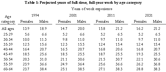
Two important predictions are made in Table 1. First the number of years of experience obtained by males at each age group will not change significantly over the next 30 years. Whereas males 45-49 had worked an average of 25.6 years in 1994, for example, they are predicted to have worked 25.5 years in 2031. Similarly, the work experience of 55-59 year-old males is predicted to change by only 0.2 years – from 36.6 to 36.8 years over the same time period.

Second, whereas the work experience of young females is predicted to remain relatively unchanged, older women are predicted to obtain more years of lifetime employment. For example, while the work experience of 35-39 year-old females is predicted to change by 0.1 years between 1994 and 2031 – from 12.5 to 12.4 – the work experience of 55-59 year-olds is predicted to increase by 2.3 years – from 23.9 to 26.2. And the experience of 60-64 year-olds is predicted to increase by 5.1 years.

Shannon and Kidd concluded that these changes will produce only a slight narrowing of the wage gap between men and women – and then only in older age groups. But their results did not allow for changes in number of hours worked in a lifetime. It is also possible that some wage gains could be obtained by women if they were to work more full-time hours, and less part-time, and if they were to increase their full-time hours. In 1997, for example, women working full-time, worked 39 hours per week on average, whereas men worked 43 hours.

Shannon and Kidd incorporate the trends summarized above to determine the future wage gap. Their results are shown in Table 2 below.

Figure 2

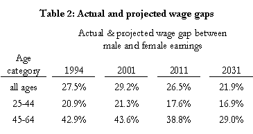
There, it is projected that the gender wage gap will decline in the future. On average, it is projected that the difference between incomes for males and females in the 25-44 year age category will fall to approximately 17 percent by 2031. That is, full-time, full-year wages for females within the 25-44 year age category are projected to be approximately 83 percent of their male counterparts. By comparison, women in the 45-64 year age group will earn approximately 71 percent of their male counterparts’ incomes.

Conclusions & implications

Shannon and Kidd’s results imply that the gender wage gap will continue to close, but a gap of approximately 22 percent will still exist in 2031. Increasing female labour force participation and educational attainment, coupled with the relative stability of the male labour force participation and education attainment contribute to the wage gap closure.

In comparison to the wage gap closure from 1967 to 1997 (42 percent to 27 percent, or 15 percentage points), the results for the next three decades suggest that convergence of the gender wage gap will slow from 2001 to 2031 (29 percent to 22 percent, or 7 percentage points). The authors’ findings also suggest that changes in the wage gap for older individuals (within the 45-64 year age group) will produce the greatest convergence (43 percent to 29 percent, or 14 percentage points).

Part of the projected wage gap in 2031 is due to the differences in the labour market characteristics addressed by Shannon and Kidd. Since women tend, on average, to work fewer years over their work-life; work fewer hours per week; and are more likely to withdraw from the labour force or reduce their hours to part-time for the purposes of raising a family, their wages will, on average, be less than those of their male counterparts. However, these characteristics historically have accounted for only half of the wage gap. The portion of the wage gap that cannot be explained by labour market characteristics is generally attributed to discrimination and to differences in preferences between men and women. For example, women tend to be the primary caregivers. Thus, they may choose to work in lower-paying jobs that have more flexibility regarding sick days and hours worked, or within positions that are easily entered and exited. These are factors which also contribute to the wage gap, but are not easily captured using traditional statistical methods, such as those used by Shannon and Kidd.

What do these findings imply for using male earnings when predicting the potential income for young females? It seems reasonable to conclude that the findings suggest that historical average income figures for women underestimate the future potential income of an average young woman today. This is because historical income figures reflect women who (on average) had a much different labour force experience than today’s average young woman will experience, and that young women in the future will experience. It seems that the “reality” for today’s average woman lies somewhere between historical figures for males and females. It appears that even young women who will follow a “traditional” average female career path will earn more than the average women represented by historical data since today’s females are acquiring higher education levels and displaying a greater labour force attachment by participating full-time in the labour force longer.

Thus, it may be appropriate to use average earnings for males to predict the future potential income of an average young female, and then to apply contingencies to reflect the possibility of labour force absences and part-time employment. I emphasize, however, that this approach still carries difficulties. For example, women tend to enter different careers than men, even when they are working full-time. That is, there is still a tendency for occupations to be “male-dominated” or “female-dominated”, and the female-dominated occupations tend to pay less, even considering the same level of educational attainment between men and women. Thus, using male earnings data for any given level of education (considering all occupations) may overstate the potential life-time earnings of a young female.

Footnotes

* Shannon, Michael and Michael Kidd, 2001, “Projecting the Trend in Canadian Gender Wage Gap 2001-2031”, Canadian Public Policy. Vol. XXVII, No. 4, 447-467. [back to text of article]

** Shannon and Kidd also consider a scenario in which enrolment increases in the future at the same rate it had increased in the prior 12 years. For the purposes of this article, I focus on the more conservative scenario in which they assume that there is a one-time jump in enrolment from 1994-2000, and then enrolment remains constant over the 2001-2031 period. [back to text of article]

leaf

Kelly Rathje is a consultant with Economica and has a Master of Arts degree (in economics) from the University of Calgary.

Complementarity in the Retirement Behaviour of Older Married Couples: An Update

by Daryck Riddell & Christopher Bruce

This article first appeared in the spring 2002 issue of the Expert Witness.

When forecasting the earnings streams of individuals over 50, one of the most important factors is predicted age of retirement. For example, changing the projected retirement age from 63 to 60, when the individual is currently 57, will decrease the future loss of earnings by approximately 50 percent.

It is often argued that one indicator of likely retirement age among individuals in this age group is the retirement decision of the plaintiff’s spouse. If a 57 year-old woman’s husband has already retired, that could indicate that she will retire earlier than would otherwise have been predicted.

Economists have observed three factors that might suggest a correlation between the retirement ages of spouses. These we refer to as: similarity of profiles, sharing of household finances, and complementarity of leisure.

Similarity of Profiles

Sociologists, psychologists, and economists have long observed that individuals choose mates who have socio-economic profiles similar to their own. If professionals marry professionals or high school leavers marry high school leavers, then the retirement ages of spouses will be similar, not because the retirement decision of one spouse affected the retirement decision of the other, but because the spouses’ decisions were affected by similar work-related influences.

Spouses who both worked in physically demanding jobs might both retire earlier than the population average, for example. Or spouses who were both self-employed – say, doctors or lawyers – might both retire later than average. In such cases, one might be tempted to conclude that because one retired soon after the other that the retirement of the first had “caused” the retirement of the second when, in fact, what had happened is that they had both been affected by the same external factors.

Sharing of Income

It has long been recognised in the economics literature that the likelihood that one spouse will leave the labour market will increase as the income of the other spouse increases. That is, the spouses of high income earners are more likely to be retired at any age than are the spouses of low income earners.

This observation suggests two hypotheses. The first of these is that if one spouse’s social security benefits increase, the “other” spouse will be more likely to retire. Evidence for this hypothesis has recently been obtained in two studies. Both Coile (1999) and Baker (2002) found that both wives and husbands were more likely to retire when the wives were eligible for income supplements than when the wives were not. It appears that wives’ retirement ages, however, were not strongly influenced by husbands’ availability of income supplements.

The second implication of “sharing of income” is that spouses’ retirement ages will be negatively correlated. That is, if one spouse has retired, the other will be less likely to retire. The reason for this is that when one spouse retires, that spouse’s income decreases (often, dramatically), thereby decreasing the probability that the other spouse will leave the labour force.

Complementarity of Leisure

A third hypothesis is that spouses will obtain greater pleasure from retirement if they retire together. In economic terminology, the benefits that one spouse obtains from leisure are complementary to the amount of leisure enjoyed by the other. For example, if the wife plans to spend her retirement travelling, she may expect to obtain more pleasure from her retirement if she anticipates that her husband will also be retired and will travel with her.

Clearly, this hypothesis suggests that spouses’ retirement ages will be positively correlated. That is, if one spouse retires, the other will be more likely to retire, as the second spouse will expect to obtain greater benefits from retirement leisure than if the first spouse had not retired.

Blau (1998) has recently provided evidence that this complementarity is an important factor in determining spouses’ retirement ages. His study examines the joint labour force behaviour of older married couples in the United States.

Using the Retirement History Survey (RHS), a longitudinal study that followed men and women who were age 58-63 in 1969, Blau constructs labour force histories for each married couple from the time the husband turned 55. The joint labour force status of the couple in any given time period is characterized by four possible states: both employed, neither employed, husband employed but wife not, wife employed but husband not.

The data set has some interesting features. Foremost among them is that the labour force transitions of one spouse are strongly associated with the labour force status of the other spouse. The wife’s exit rate from the labour force is 63 percent higher when the husband is not employed than when he is employed. Similarly, the husband’s exit rate when his wife is not working is 53 percent higher than when she is employed. Conversely, quarterly entry rates for both husband and wife are larger if the other spouse is employed rather than not employed.

Another feature is that the incidence of joint retirement is quite large. Between 11.4 percent and 15.7 percent of all couples exit the labour force in the same quarter and between 30.3 percent and 40.6 percent exit in the same year.

The key conclusion from this paper is that there is strong evidence of the preference to share leisure. This sample from the 1960s and 1970s shows a high incidence of joint retirement and a positive effect of non-employment of one spouse on the other spouse’s labour force exit rate, as well as a negative influence of non-employment of one spouse on the other’s entry (or re-entry) rate.

Summary

Economists have put forward three hypotheses concerning the likelihood that the retirement ages of spouses will be correlated. The first of these – similarity of profiles – suggests that, on average, spouses will retire at similar times because spouses tend to have similar socio-economic profiles. That is, the factors that act on retirement age independently of marital status will affect husbands and wives in similar manners.

The second hypothesis is that individuals will be more likely to retire, the higher is their spouse’s income. This hypothesis suggests that there will be a negative correlation between spouses’ retirement ages. When one spouse retires, family income will decrease and the second spouse will be provided with an incentive to remain in the labour force.

Finally, if the leisure activities of husband and wife are complementary, there will be a positive correlation between spouses’ retirement ages. Recent evidence suggests that this effect has been a significant determinant of retirement ages in the United States.

leaf

Daryck Riddell was a graduate student in Economics at the University of Calgary

Christopher Bruce is the President of Economica and a Professor of Economics at the University of Calgary. He is also the author of Assessment of Personal Injury Damages (Butterworths, 2004).