Mathematical Mistake: Averaging Multiple Statistical Sources Together to Form One “Overall” Average Income Figure

Posted on March 1, 2008March 26, 2017 By economica

This article first appeared in the spring 2008 issue of the Expert Witness.

In estimating a plaintiff’s without- or with-incident income, there is a mathematical mistake that an economist can make that will potentially have a large impact on the resulting income path and, subsequently, on the plaintiff’s loss of income. This mistake is the practice of averaging multiple statistical sources together to obtain one “overall average”. It may seem reasonable, at first glance, to assume that averaging multiple sources of statistical data would result in an overall average which is superior to the quality of the individual averages. However, this is often not the case. This approach can lead to an incorrect and misleading estimate of a plaintiff’s income due to double-counting, a failure to take into account differing quality of each source (as measured by sample size), and the inclusion of important characteristics (such as age, education, and gender) that are not applicable to the plaintiff. This method also has the potential to provide misleading estimates simply based on the choice of the sources used in calculating this “average”.

To illustrate these effects, we have summarized in the table below, the average income for partsmen (as an example) obtained from a number of common statistical data sources.

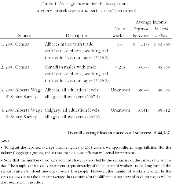
Table 1

As shown in the table, if we were to “average” across all of the incomes then we would get an income figure of $44,567 (in 2008 dollars). However, this would be an incorrect and potentially misleading estimate of the average income of partsmen.

The first reason the above “average” figure is incorrect stems from a form of double-counting. Notice that sources one and three provide the average income of partsmen in Alberta, source two provides the average in the whole of Canada, and source four provides the average income of partsmen in Calgary. However, the Alberta data from source one are already included in the Canadian data from source two. Similarly, the Calgary data from source four are already included in the Alberta data from source three. Thus, the average incomes reported by sources one and four are based on data that were already present in sources two and three. Additionally, because the data from sources one and four are already included in sources two and three, these sources have been included in the overall average figure twice. This double-counting is mathematically incorrect and can lead to biased estimates of a plaintiff’s income (i.e. estimates which are either higher or lower than the actual average income). For example, if we were to use only the sources for Alberta overall (and exclude the sources for Calgary and for Canada overall), we would obtain an average income of $47,023 (or approximately $2,456 more than the “overall” average). Thus, taking an average across multiple sources of statistical data will lead to double-counting, and thus to biased estimates of a plaintiff’s income, due to this overlapping of data from a variety of sources (i.e. data from Canada includes data from Alberta, which in turn includes data from Calgary).

The second reason that taking an average across all of the sources is incorrect is that we have not accounted for the “quality” of each source, measured in this case by the size of the sample upon which the average income from each source is based. For example, we have applied equal weight to source one, whose average income was obtained using data from a Statistics Canada survey of approximately 179 workers (about one-fifth of the reported “number of workers” figure), as to source two whose average income was obtained using data from about 843 workers (almost five times as many as source one). In addition, we have taken an average that includes sources whose sample size is unknown. As an example, and ignoring the “double-counting” problem for a moment, if we were to take a simple average of sources one and two, we would get an overall average of $49,635 (= [$53,960 + $45,309] ÷ 2). However, if we were to calculate a proper average that takes into account the different sample size of each source, we would get an average income of $46,824 (= $53,960 × 895 / 5,110 + $45,309 × 4,215 / 5,110), or approximately $2,810 less than the simple average. Thus, taking a simple average across multiple sources of statistical data will lead to biased estimates of the plaintiff’s income, due to a failure to account for varying sample sizes across the different statistical sources.

The third reason that taking an average across multiple sources of statistical data is incorrect is that this figure includes income data from partsmen of varying education levels and gender. That is, (setting aside the double-counting and sample size problems for a moment), sources one and two provide average incomes for males with a trade certificate/diploma, while sources three and four are comprised of data for partsmen of all education levels, as well as from data for both male and female partsmen. Essentially, each of these sources provides income data for individuals who are not comparable to each other (the “apples to oranges” problem).

For example, the “overall” average figure combines the average income of partsmen with trade certificates or diploma with partsmen of all education levels. The partsmen with formal post-secondary training in their field will be expected to earn more than partsmen of all educations, since the latter group will include some workers without formal training. Thus, including the all-educations categories will bias the overall average downward if we are attempting to estimate the average income of partsmen with formal post-secondary training in their occupation. (And similarly, if we are attempting to estimate the average income of partsmen without formal post-secondary training, then including categories one and/or two will bias the average upwards.) Additionally, by including sources three and four, we have included data from female partsmen and from partsmen with varying levels of education. Thus, by taking an average across all sources, we have incorporated a variety of important characteristics (such as location, education, and gender) which may not be applicable to the plaintiff and which could significantly bias the resulting estimate of the plaintiff’s income.

Finally, the approach of taking an average across multiple sources of statistical data has the potential for allowing estimates to be biased upwards, or downwards, simply by choosing the sources that are included in the average. For example, we have included the 2001 Census and the 2007 Alberta Wage and Salary Survey in Table 1 and obtained an “overall” average of $44,567. Suppose we also found one survey that indicated an average income for partsmen of $60,000 and one survey that indicated an average income of $35,000. If both of these new sources were included in the “overall” average (and ignoring the double-counting, sample-size, and characteristic problems for the moment), we would calculate a new average of $45,545, which is close to our original average. However, if we chose to only include the $60,000 survey, our new average would be $47,653. Alternatively, we would obtain an average income of $42,653 by only including the $35,000 survey. In other words, one could potentially obtain an estimate of a plaintiff’s income which is biased upwards, or downwards, by simply altering the selection of sources. The fact that this method is open to this potential form of abuse suggests that this approach should not be used.

In summary, taking an average across multiple sources of statistical data can lead to biased estimates of a plaintiff’s income due to the double-counting of data, the failure to take into account differing sample sizes, and the inclusion of important characteristics (such as geography, age, education, and gender) that are not applicable to the plaintiff. In addition, this approach has the potential for abuse in that the estimate of a plaintiff’s income can be biased upwards or downwards by the selection of the statistical sources used in the calculations. Note that it may be difficult to detect these problems if the sources have not been adequately described or if the reader is not familiar with the sources or methodology used in calculating the average. A better approach would be to rely on one, high quality, well justified data source (such as the Canadian census). This avoids the many problems associated with combining multiple sources and does not open the door to using various sources to obtain a higher or lower estimate of a plaintiff’s income.

Laura Weir has a Bachelor of Arts in economics (with a minor in actuarial science) and a Master of Arts degree from the University of Calgary. She has worked for Economica since 2006.

The Impact of Childhood Sexual Abuse on the Educational Attainment and Adult Earnings of Canadian Women

Posted on September 1, 2007March 26, 2017 By economica

The Impact of Childhood Sexual Abuse on the by Christopher J. Bruce, Ph.D. & Daniel V. Gordon, Ph.D.

This article first appeared in the autumn 2007 issue of the Expert Witness.

Introduction

One of the most complex issues facing the courts in any sexual abuse case is the determination of the impact that the harm has had on the plaintiff’s earning capacity. Not only is very little statistical evidence available on this issue, but the data that do exist have often proved to be unreliable.

Recently, this lack of a reputable source has been resolved with the publication of a Statistics Canada survey in which a representative sample of Canadians was asked about their experiences of victimization. From this survey, we were able to obtain information about a large set of (adult) women who had suffered sexual abuse as children.

The purpose of this paper is to report our findings concerning the consequences of that abuse on the educational attainment and earnings of the victims. Our surprising result is that, among most such victims, abuse does not have a statistically significant effect on adult education and earnings. Furthermore, in the only group for which abuse
was found to have a significant effect – women who were first abused between the ages of seven and thirteen
– education and income were higher than among women who had not been abused.

The remainder of the paper is divided into three sections: a review of the existing literature; the development of an economic model concerning the effect of abuse; and a summary of our statistical findings.

Existing Literature

The academic literature concerning the effects of childhood sexual abuse is composed of two streams. In the first, researchers have attempted to develop theories of childhood social-psychological development that can be used to understand the pathways by which abuse affects its victims. In the second, researchers have used statistical tests to identify correlations between abuse and its predicted outcomes, such as depression, alcoholism, and school completion rates.

Theoretical

Many theories concerning the impact of sexual abuse are founded on the ‘core-symptom’ model, in which a
core problem or event is presumed to have led to one or more symptoms. The most common of these models characterize sexual abuse as a trauma, leading researchers to predict that abuse will result in post traumatic stress disorder.

An alternative interpretation suggests that, rather than
having a single effect, sexual abuse might produce multifaceted effects. Finkelhor and Browne (1985), for example, argued that sexual abuse had four primary effects: traumatic sexualization, stigmatization (i.e. low esteem and self-destructive behaviour), betrayal, and powerlessness.

A third approach, ‘developmental models,’ proposes that sexual abuse may affect victims by interfering with development in areas such as social- and self-functioning. In this view, therefore, the age at which the child is abused may be a critical determinant of the long-term effects of that abuse. For example, Celano (1992) suggested that the impact of sexual abuse may differ among Piaget’s three stages of childhood moral development (Piaget, 1965): preschool (ages 0-6), latency (7-13), and adolescence (14-19). She hypothesised that whereas preschoolers may not recognise that abuse is morally reprehensible, and adolescents may consider their moral culpability to be ameliorated by failure to provide informed consent, children in the latency period may consider themselves (at least in part) to be responsible for many of the types of abuse. Accordingly, she predicts that abuse will be most harmful if it occurs in the latency period.

Statistical

Statistical studies can roughly be divided among those that investigate the effect of sexual abuse on: psychological factors, (such as depression, self-esteem, and sexuality); social outcomes, (such as alcoholism and delinquency); and economic outcomes, (specifically, schooling and adult income).

This literature is virtually unanimous in its finding that childhood sexual abuse has statistically significant effects on the victim’s psychological well-being. The outcomes that are most commonly found include: low self-esteem, post-traumatic stress disorder, depression, affective and personality disorders, and anti-social behaviour.

The sociological literature has provided evidence concerning the effect that abuse has on criminal activity. Studies that aggregate across a number of different types of childhood abuse
– neglect, physical abuse, and sexual abuse, for example
– commonly find that criminal activity is correlated with
this aggregate; although some find no statistically significant correlation. Importantly, however, when ‘abuse’ is separated into its components, it is only ‘neglect’ that is found to be correlated with criminal activity. Neither physical nor sexual abuse appears to be a significant determinant in this formulation.

Very mixed results have been obtained when researchers investigate the impact of abuse on schooling and income. Slade and Wissow, (2006) found that individuals who had been maltreated as children had lower high school GPAs than the control group, but no greater problems with teachers, with completion of homework, or with school absences. And some studies have found evidence that victims of childhood sexual abuse performed better in school than those who had not been abused (e.g. Eckenrode, et al. 1993 and Buckle, et al. 2005).

Economic Model

In our model, we assume that individuals divide their time among three activities: solitary leisure activities, such as reading, watching television, and playing video games; social leisure activities, such as team sports, club memberships, and interacting with friends; and “market” activities, such as investing in education and working in the labour market. The value of each activity increases as additional time and effort is devoted to it. And the “cost” of time spent in any one activity is the value that is foregone from the other activities (the “opportunity cost” concept so familiar to economics students).

We hypothesize that the effect of sexual abuse is to reduce the benefits that individuals obtain from each of the three activities. Normally, one would expect that this would lead to a reduction in each of them. However, assume that the negative effect on the time and effort devoted to two of the activities was greater than it was on the remaining one. In that case, it is possible that the victim might “substitute” away from the more seriously-affected activities towards the less-seriously affected one. As a result, the latter might even increase.

For example, if abuse had a much more significant (negative) impact on the individual’s ability to socialize than on
her ability to undertake schoolwork or to compete in the labour market, abuse might lead to a lesser reduction in the latter activities than expected, and could even lead to an increase in those activities. In common parlance, the individual might be said to have compensated for the harm to her socialization skills by ‘throwing herself’ into academic and work-related activities. In such a case, abused individuals might be observed to complete more years of education than the non-abused, and might earn higher incomes; but this would come at the expense of a significant withdrawal from normal social activities. We propose to test for this effect in the analysis reported in the next section.

Statistical Estimates

We obtained information concerning 6,528 adult Canadian
women, (drawn from the 1999 General Social Survey), of whom 607 reported that they had been sexually abused as children. Using the data from this survey, we conducted two statistical tests.

In the first of these, we estimated the effect of a series
of variables on educational achievement. The variables that are usually found to be important – such as parents’ education, individual’s place of birth, and whether the individual belonged to a “visible minority” – all proved
to be significant in our data. In addition, we found that if the individual had first been sexually abused between the ages of seven and thirteen, she obtained more education than did individuals who had not been abused or who had first been abused before seven or after thirteen.

In our second test, we estimated the effect of a number of background variables on adult earnings. As expected, we found that variables such as the individual’s education and whether she belonged to a visible minority had significant effects on income. And, again, we found that individuals who had been abused between the ages of seven and thirteen had statistically higher levels of income than did those who had not been abused or who had first been abused before seven or after thirteen. Importantly, this effect is in addition to the increase in income that would have arisen from the effect of abuse on education.

To summarise, we found: first, that abuse before the age of seven or after the age of thirteen had no statistically discernable effect on either the victim’s education or her adult income. Second, abuse between the ages of seven and thirteen increased average educational levels and increased average incomes, both directly and indirectly (through the effect on education).

Conclusion

We have found that, on average, sexual abuse is not associated with lower educational levels or lower adult incomes among victims. This does not mean that all victims have higher income levels than those who have not been victimised: some victims will be above-average and some below. When the court is dealing with a particular plaintiff, it should always rely on factors that are specific to that individual. Nevertheless, our results suggest that it cannot be concluded, without such specific information, that the individual’s adult income will be adversely affected by sexual abuse.

References

Buckle, S., S. Lancaster, M. Powell, and D. Higgins (2005) “The Relationship Between Child Sexual Abuse and Academic Achievement in a Sample of Adolescent Psychiatric Inpatients,” 29 Child Abuse and Neglect, 1031-1047.

Celano, M. (1992) “A Developmental Model of Victims’ Internal Attributions of Responsibility for Sexual Abuse,” 7 Journal of Interpersonal Violence, 57-69.

Eckenrode, J., M. Laird, and J. Doris (1993) “School Performance and Disciplinary Problems Among Abused and Neglected Children,” 29 Developmental Psychology,
53-62.

Finkelhor, D., and A. Browne (1985) “The Traumatic Impact of Child Sexual Abuse: A Conceptualization,” 55 American Journal of Orthopsychiatry, 530-541.

Piaget, J. (1965) The Moral Judgement of the Child, (New York: Free Press).

Slade, E., and L. Wissow (2006) “The Influence of Childhood Maltreatment on Adolescents’ Academic Performance,”
Economics of Education Review, (in press).

Christopher Bruce is the President of Economica and a Professor of Economics at the University of Calgary. He is also the author of Assessment of Personal Injury Damages (Butterworths, 2004).

Daniel V. Gordon, Ph.D., is a professor of economics at the University of Calgary, where he specialises in the use of statistics for economic analysis.

Using the HALS/PALS data sets to estimate a loss of income

Posted on March 1, 2007March 26, 2017 By economica

by Derek Aldridge

This article first appeared in the spring 2007 issue of the Expert Witness.

Many of our readers will have heard of Statistics Canada’s “HALS” and “PALS” disability statistics. These result from surveys that collected data concerning Canadians with disabilities and the manner in which their everyday lives are affected by these disabilities. The HALS statistics are from Statistics Canada’s 1991 Health and Activity Limitation Survey and the PALS statistics are from the 2001 Participation and Activity Limitation Survey.

Of particular interest to our readers is how these statistics can be used to predict the economic impact that a particular disability will have on a specific plaintiff. I have been asked numerous times by plaintiff’s lawyers if it is possible to use the HALS statistics to help determine their client’s loss. In addition, I have been asked by defence lawyers to rebut the claims of other economists who have used this approach. In this article I will discuss the difficulty of using the HALS/PALS approach to estimate a plaintiff’s loss of income. Before offering my comments concerning these statistics, I will provide some background information on the data sets.

In the 1991 and 2001 censuses, recipients of the long-form census forms were asked a few questions designed to determine whether or not they were disabled in a way that limited their activities at home, at work, or at school. Some of those who indicated a disability were subsequently interviewed for a detailed disability survey (a “post-censal” survey). Following the 1991 census, approximately 35,000 adults from the “disabled” census group were selected for the detailed HALS survey. (For technical reasons that do not need to be discussed here, a larger number from the “non-disabled” census group were also selected for the follow-up survey.) Following the 2001 census, approximately 35,000 adults and 8,000 children from the “disabled” census group were selected for the detailed PALS survey.

The 1991 HALS survey identified six types of activity limitation among the adults surveyed: hearing, seeing, speech, mobility, agility, and other (a grouping of non-physical disabilities related to psychological conditions, learning, memory, and so forth). The 2001 PALS survey identified ten types of limitation: hearing, seeing, speech, mobility, agility, learning, developmental disability or disorder, psychological, memory limitation, and chronic pain. Individuals were asked questions to determine the degree of their disability and based on the answers to these questions, their level of disability was assigned a severity scale. In 1991 there were three severity levels: mild, moderate, and severe. In 2001 the severity levels (except for children under five) were mild, moderate, severe, and very severe. The classification examples below are from the Statistics Canada Publication A Profile of Disability in Canada, 2001 (Catalogue 89-577-XIE):

For example, a person who has no difficulty walking and
climbing stairs but cannot stand in line for more than 20
minutes, would have a mild mobility-related disability. A
person who can only move around in a wheelchair would have
their mobility more severely limited, and one who is
bedridden for a long term period would have a very severe
mobility-related disability. The number of disabilities also
has an impact on the overall level of severity. The PALS
distinguishes 10 types of disabilities among adults and the
level of severity will increase with the number of
disabilities affecting each individual. [Pages
19-20]

In addition to questioning individuals about their limitations, PALS also asked about the cause of disability (e.g., a motor vehicle accident), the age at which the activity limitations began, the level of education, the number of hours worked per week, the reason for working fewer than 30 hours per week, the person’s occupation and industry, the rate of pay, the amount of unemployment experienced in the past year, and numerous other questions. The PALS questionnaire and reporting guide is 86 pages long.

As a result of these surveys, there is a wealth of information available concerning people with disabilities in Canada. Some examples follow, again taken from the publication A Profile of Disability in Canada, 2001:

Mobility problems are the type of disability most often
reported by adults aged 15 and over. In 2001, nearly 2.5
million or 10.5 percent of Canadians had difficulty walking,
climbing stairs, carrying an object for a short distance,
standing in line for 20 minutes or moving about from one room
to another.
More than 10 percent of adults have activity limitations
related to pain or discomfort.
The prevalence of most types of disabilities increases
with age.
A large majority of persons with disabilities aged 15 and
over have more than one disability.
Nearly 6 percent of Canadians aged 15 and over have a
severe or very severe disability.
7.5 percent of all working-age persons are limited in
their activities due to pain or discomfort.

This is all very interesting, and surely the survey results have many useful applications. However, for our purposes, we want to know how these surveys can be used to help estimate a specific person’s loss of income as a result of an injury. A statistical (econometric) analysis of the data could tell us (for example) how the annual income of an average “severely disabled” male differs from that of males overall. Even better, we might be able to compare the incomes of male journeyman welders age 30-40 who are experiencing severe pain and agility disabilities, with the corresponding average for those who are not disabled. (Or with the corresponding overall average that includes mostly people who are not disabled, and some who are.) Note however, that we have a problem in that as we get more and more specific with respect the category of disabled people, we have less and less confidence in the accuracy of the reported averages. This is because as we get more specific, our sample size gets smaller and smaller and the characteristics of the sample become heavily influenced by the characteristics of a few individuals. I think we could be reasonably confident in our claims about the earnings of severely disabled males relative to males overall, but not very confident at all about my hypothetical welders.

For now let us ignore the technical problems that might arise, and suppose that we are able to construct a statistical model with the HALS data and use it to estimate with confidence, the average earnings of full-time employed severely disabled males aged 30-40 with high school diplomas. Suppose we find that they earn 25 percent less than the overall average for full-time employed males aged 30-40 with high school diplomas. How can we use this information when we come upon a 35-year-old plaintiff who is a high school graduate and has residual deficits that can be categorised as severe? Suppose the plaintiff is working as a full-time truck driver, and we determine that he is earning about 25 percent less than the average for truck drivers his age (consistent with the HALS prediction). Perhaps we can now conclude that the HALS approach does a fine job of predicting his loss of income, assume that the 25 percent loss will continue until retirement, calculate the present value, and move on to the next case.

This conclusion might be reasonable, but what if it is found that the plaintiff can improve his income by retraining and changing occupations? What if it is found that his condition will improve (or worsen) in the future? What if we find that he was already earning a below-average income before he was injured? My point here is that while it is useful to consider the average impact of disability, it is more important to examine the specific plaintiff at hand and investigate how his injuries are affecting his employability and his income. With respect to these issues, the advice of a vocational expert can often be especially helpful.

It is important to recognise the meaning of my (hypothetical) 25 percent reduction estimate, and its limitations. I proposed that the evidence might support a conclusion that full-time employed severely disabled 30-40 year-old males with high school diplomas earn 25 percent less than their non-disabled counterparts on average. In other words, if we randomly selected from the population a person in this category, we would predict that his income will be 25 percent less than the average for his non-disabled counterparts. However, once we can more closely examine the randomly chosen person, we learn more information about him and we may need to revise our prediction.

For example, suppose he has a severe mobility disability but he is also a professional writer. In this case we might have to revise our prediction since his earnings as a writer are probably only slightly affected by his poor mobility. What if we learned that he had been a professional hockey player but had to leave that occupation and is now working in sales? In this case we would also revise our prediction since his earnings reduction is likely much more than 25 percent. It should be clear that as soon as we are considering a particular individual, and not some unknown “randomly selected” person, we need to try to incorporate the additional information we have about that person, and if our HALS estimates are no longer sensible, they should be discarded. This principle is the same as would apply if we wanted to predict the income of a full-time 45-year-old female teacher who is at the top of the salary grid with the Calgary Board of Education. It would be foolish to rely on census data for female teachers instead of simply consulting the appropriate salary grid.

In most cases, it is not even necessary to concern ourselves with the predictions of a HALS model. If a plaintiff was a well-established welder and now he is unemployable due to an injury, HALS adds nothing to the estimate of his economic loss. However, suppose we have an individual whose disabilities are categorised as severe, but he continues to work in his pre-accident job and is not currently experiencing a loss of income. Might this be an occasion when the HALS approach is especially useful in estimating his loss of income, due to the uncertainty regarding how his injuries will affect his future earnings? Probably not. To begin with, the fact that the plaintiff is not currently experiencing a loss of income suggests that he is unlike the average HALS individual. It is an awkward but unavoidable fact that a statistical model will not do a good job of predicting outcomes for “outliers”. That is, if we create a predictive statistical model using a certain sample group, the model’s predictive power diminishes if the subject under consideration is very much unlike the average member of the sample group. But let us ignore this problem for now.

Perhaps we could assume that, in the future he will be more like the average and will experience that 25 percent loss, on average over the remainder of his work-life. This immediately leads to a logical problem that should give plaintiff lawyers pause before relying on such an assumption. If one wants to argue that a plaintiff who is not now experiencing a loss of income will become just like the HALS average in the future, then what of the plaintiff who is now experiencing a loss of income greater than the predicted 25 percent? The reasoning above suggests we should assume that his earnings will improve to only a 25 percent loss, on average, over the remainder of his work-life. This reasoning is, of course, faulty. When we observe a person experiencing less than the expected income reduction, the reasonable conclusion is that he is one of the individuals whose disability has a relatively mild effect on his earnings. The conclusion is not that his earnings gap will widen in the future, as this effectively ignores the additional information conveyed by the his current income. Parallel reasoning applies when we have a person experiencing a greater than expected income reduction.

To be clear, it could be the case that the working plaintiff who is not currently experiencing a loss of income will indeed experience one in the future. However, I do not believe that the loss will be supportable using HALS alone. In such a case, the HALS data would tell us that the individual is currently performing better than his disabled peers (on average), but we still need more evidence to find that he will have a future loss. That evidence may be available from medical experts, vocational experts, or the plaintiff’s employer. Perhaps there is evidence that the plaintiff faces a greater chance of future unemployment, or is likely to retire early due to his residual deficits. These factors will lead to a loss of income and they can be explicitly incorporated in our calculations – there is no need to appeal to HALS averages. Alternatively, it may be the case that the plaintiff is not now experiencing a loss of income because the injuries are not affecting his ability to earn income and never will. In that case we might be left with a “loss of capacity” argument, which I will not address here.

To summarise, I believe that in most cases when we have an adult plaintiff, the HALS approach is not going to be especially useful in determining his loss of income. It simply provides a useful baseline to compare a particular plaintiff to his disabled peers, in the same way that census income averages tell us how a particular 45-year-old female teacher’s earnings compare to her same-age peers.

There are cases in which I think the HALS approach could be useful, and these are when we know very little about how a disability will affect a person’s employment and earnings. For example, in the case of a child who is injured, we could use HALS to predict the impact on her future earnings. Even in such circumstances, the HALS approach would still be limited in at least two ways. First, the HALS approach will only be valid if the child’s expected educational attainment is unaffected by the injuries. Second, in such a case we would also need a HALS model that can be restricted to those adults who were injured when they were children, since there will certainly be a difference in the impact of (say) a severe mobility disability on earnings if the person is injured at age 10 versus if she is injured at age 40. This restriction will add to the sample size problems I noted above. For an injured adult the HALS approach could be useful if there remains a great deal of uncertainty regarding how her earnings will be affected. For example, in the case of a plaintiff who has been out of the labour force for many years (due to parenting responsibilities perhaps) and who has not yet attempted to re-enter the labour force.

In these cases however, like all others, we must remain willing to discard the HALS averages if we have better information about how the plaintiff’s income will be affected. It is not satisfactory to say that because the loss of income is difficult to determine, HALS will yield our best estimate. In most cases we can do better, because we are not predicting the income of a randomly selected disabled individual. Instead we are predicting the income (and loss) of a specific individual about whom we know a great deal. The fact that we have a HALS model at our disposal does not mean that we should ignore the facts of our specific plaintiff.

Derek Aldridge is a consultant with Economica and has a Master of Arts degree (in economics) from the University of Victoria.

Death and Retirement: Allowing for Uncertainty

Posted on September 1, 2005March 24, 2017 By economica

by Christopher Bruce

This article first appeared in the autumn 2005 issue of the Expert Witness.

Assume that a plaintiff has begun to recuperate following a serious accident. If her injuries stabilize at their current level, she will suffer a loss of earnings of $20,000 per year. If, however, she has a relapse, her losses will increase to $40,000 per year. Her doctors tell you that there is a 50 percent chance that there will be a relapse (and a 50 percent chance that there will be no relapse).

How should the annual value of her loss be calculated? If damages are set equal to $20,000 per year, there is a 50 percent chance that she will be under compensated; whereas if she is paid $40,000, there is a 50 percent chance that she will be over compensated. (And if she is paid some amount between $20,000 and $40,000, there is a 100 percent chance that she will be incorrectly compensated.)

This conundrum, in which there is uncertainty about the outcome of future events, is common in the assessment of personal injury (and fatal accident) damages. Not only is there uncertainty about the future course of the plaintiff’s injuries, as in the example above, we also face uncertainty concerning the age at which the plaintiff will retire, the plaintiff’s life expectancy, the probability that the plaintiff would have (and will be) unemployed, and a host of other factors.

The general approach that virtually all financial experts take in such cases is to calculate the average outcome that would arise from the uncertain event, if the event could be repeated a large number of times. For example, if the injury described above was to be repeated 100 times (for example, if there were 100 plaintiffs with that same injury), we would expect that the plaintiff’s injuries would remain stable in approximately 50 cases, leading to a loss of $20,000 per case. In the other 50 cases, the plaintiff would suffer a relapse and her loss would rise to $40,000. Thus, the total annual loss, across all 100 cases, would be ((50 × $20,000) + (50 × $40,000) =) $3,000,000. The average annual loss would be $30,000; which could also be calculated by multiplying 50% times $20,000 and adding 50 % times $40,000. That is, the average value of a loss can be calculated by multiplying each of the possible losses by its probability and then adding the resulting numbers together.

But, as was noted above, $30,000 is guaranteed to be the “wrong” amount in 100 percent of cases. How, then, can it be justified? One simple answer is this: if the event in question is truly uncertain, the plaintiff should be able to use the $30,000 to purchase insurance that will compensate her fully regardless of which value turns out to be her true loss – either $20,000 or $40,000. The reason for this is that if the insurer issues, say, 100 such policies, it can expect to pay out $20,000 in 50 cases and $40,000 in the other 50, for an average of $30,000. (It will have collected $3,000,000 [= 100 × $30,000] and will have paid out $3,000,000 [= 50 × $20,000 + 50 × $40,000].)

Risk of Mortality

This type of calculation is most commonly used when dealing with the uncertainties associated with mortality. Take the extreme case in which there is a ? probability that a plaintiff will live exactly one year (and then die), a ? probability that he will live exactly two years, and a ? probability that he will live exactly three years. If he would have earned $60,000 per year but has now been left unable to work, his loss can be calculated using the technique described above. That is, there is a ? chance that he has lost one year’s income ($60,000), a ? chance he has lost two years’ income ($120,000), and a ? chance he has lost three years’ income ($180,000); for an average of $120,000 (=? × $60,000 + ? × $120,000 + ? × $180,000).

Alternatively, in such cases, it is sometimes possible to use a “rule of thumb” to estimate the loss. Given the probabilities in the preceding example, it can be shown that, on average, the plaintiff will live two more years before dying. (2 = ? × 1 + ? × 2 + ? × 3) That is, his life expectancy is two years. His expected loss can then be calculated as the sum of his losses over that life expectancy, or $120,000 (= 2 × $60,000). Note, however, that this approximation works best if the losses are approximately the same in each year, as it was here. (If the annual loss is significantly different in the first year than, say, the third year, this approach yields a biased estimate.)

What is clear is that it would be inappropriate to mix together the two calculation techniques. It is not appropriate, for example, to estimate the loss by multiplying each of the first two years’ losses by their associated probabilities and assuming that the loss continues for only two years. That would produce an “estimated” loss of only $60,000 (=? × $60,000 + ? × $120,000), $60,000 less than the true loss.

Retirement Age

The techniques described here can also be used to estimate the effect of uncertainties about the plaintiff’s retirement age. Assume, for example, that there was a ? probability that a 63 year-old plaintiff would have worked for exactly one year (i.e. to his 64^th birthday) and then retired, a ? probability he would have worked two years, to his 65^th birthday, and a ? probability he would have worked three years, to his 66^th birthday. If he would have earned $60,000 per year while working, his loss, again, can be found from the formula: ? × $60,000 + ? × $120,000 + ? × $180,000 = $120,000; or by multiplying the average number of years to retirement by his annual earnings, to produce $120,000 = 2 × $60,000.

As with the mortality example, it would clearly be incorrect to multiply each year’s earnings by the probability it would occur and assume the individual would have retired at the average age, of 65. That would produce an “estimate” of, (? × $60,000 + ? × $120,000 =) $60,000, again, only half of the correct estimate.

Christopher Bruce is the President of Economica and a Professor of Economics at the University of Calgary. He is also the author of Assessment of Personal Injury Damages (Butterworths, 2004).

Estimating the Impact of Mid-Career Retraining

Posted on June 1, 2005March 24, 2017 By economica

by Christopher Bruce and Derek Aldridge

This article first appeared in the summer 2005 issue of the Expert Witness.

Vocational psychologists commonly recommend that injured plaintiffs retrain for a new occupation. A problem that this creates for the financial expert is that it is not clear what the individual’s starting wage will be once the training period has been completed.

Specifically, all of our data concerning incomes by occupation suggest that individuals’ incomes increase as they age (usually until their mid-40s). If we assume that this increase occurs either because individuals gain valuable experience in their occupations or because they move up “career ladders” as they age, individuals who change careers will find themselves starting at lower wages than would be suggested by their ages.

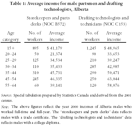
For example, Table 1 reports incomes by age (for Alberta males) for two occupations that are commonly recommended as retraining possibilities: partsman (NOC-S B572) and drafting technologist/technician (NOC-S C153). It can be seen there that annual incomes rise continuously from the youngest age group, 20-25, to the second oldest group, 45-54, before declining slightly.

Table 1

If it has been recommended that, say, a 40 year-old male retrain to enter one of these occupations, the economic expert is faced with determining which of the income levels from Table 1 best represents the income at which the plaintiff will begin his new career. If experience in the occupation, or movement along a career ladder, are important determinants of income, then we would expect that the newly-trained worker would begin at one of the lower incomes suggested by the census data.

Perhaps with his greater maturity the 40 year-old would not start at the income level of a 20-25 year-old; but with no experience in this occupation, it seems unlikely that he would start at the income of a 40 year-old. Fortunately, statistical evidence has recently become available that can help us to determine the impact of a change in career.

Most importantly, Arthur Goldsmith and Jonathan Veum[*] have used a detailed survey that followed 1400 young workers from 1979 to 1996 to compare the effects of additional years of experience on wages when individuals: remained in the same occupation and industry, remained in the same occupation but moved between industries, remained in the same industry but changed occupations, and changed both occupations and industries.

What they found was that the value that was placed on previous experience was approximately the same for all individuals except those that had changed both occupation and industry. In their words:

…experience acquired while a real estate agent is
valued similarly as tenure at other occupations, such as
accounting, within the real estate industry. In addition, the
experience as a real estate agent is valued similarly to
tenure at other industries, such as the pharmaceutical
industry, if continuing in the occupation of sales. If the
real estate agent becomes an accountant in the pharmaceutical
industry, however, the experience as a real estate agent is
of less value than that within accounting or the
pharmaceutical industry. (p. 442)

Referring to the examples in Table 1, Goldsmith and Veum’s findings suggest that the 40 year-old who retrains as a partsman may be able to earn an income comparable to that of a 40 year-old partsman with 15 years experience, if the retrained individual remains within his previous industry. For example, if an individual who had previously worked on oil rigs becomes a partsman in a shop that provides equipment to oil rigs, he can be expected to obtain a starting salary much higher than he would have obtained if he had become a partsman in an automobile dealership.

We would suggest that Goldsmith and Veum’s findings be interpreted in the following way: First, if the plaintiff’s injuries require that he/she retrain for both a new occupation and a new industry, the starting salary should (normally) be selected from the 25-29 year-old census category. This allows for the finding that previous experience is of limited importance, while avoiding the confounding effect that the incomes of 20-24 year-olds will be biased downwards by issues of immaturity.

Second, if the plaintiff’s injuries require that he/she retrain for a new occupation in the same industry he/she worked in prior to the accident, it should be assumed that the experience gained in the previous occupation will be, in large part, transferable to the new occupation. This does not necessarily mean that a 40 year-old plaintiff should be assumed to start his/her new career at the income level of an experienced 40 year-old in that occupation. Most importantly, plaintiffs often experience residual mental and physical difficulties that will reduce their earning capacity below that of the individuals represented in the census data. Also, however, it must be recognised that Goldsmith and Veum’s results referred to individuals who had changed occupations voluntarily; that is, to individuals who had chosen new occupations that met both their interests and their aptitudes. Plaintiffs often are not provided with that opportunity. As the new occupations for which they are retraining are not those that they had chosen when they were healthy, it is possible that they will not perform as well as individuals who had chosen those occupations voluntarily.

Finally, it must be recognised that Goldsmith and Veum’s findings are only suggestive. They can only be interpreted to indicate that, on average, when uninjured individuals make mid-career changes within a given occupation or industry, they tend not to suffer appreciable losses of earnings. They provide less information about specific individuals, particularly those who make significant career changes because of injury. We strongly suggest, therefore, that counsel request an opinion from a vocational psychologist concerning the impact that the injuries suffered by the particular plaintiff in question will have on that individual’s earning capacity. Specifically, if the psychologist recommends that the plaintiff retrain for a different occupation or industry, does the psychologist believe that that individual will be able to begin the new career at a salary that is comparable to other individuals of his/her age? Or will the plaintiff be forced to enter the new career at a salary lower than that of otherwise comparable individuals?

Footnotes

* Goldsmith, A.H. and J.R. Veum (2002). Wages and the Composition of Experience. Southern Economic Journal, 69(2), 429-443. [back to text of article]

Christopher Bruce is the President of Economica and a Professor of Economics at the University of Calgary. He is also the author of Assessment of Personal Injury Damages (Butterworths, 2004).

Derek Aldridge is a consultant with Economica and has a Master of Arts degree (in economics) from the University of Victoria.

Using family background to Predict Educational Attainment in Canada

Posted on September 1, 2004March 24, 2017 By economica

by Carmen Anderson with Christopher Bruce

The article first appeared in the autumn 2004 issue of the Expert Witness.

Introduction

It is important, when predicting the lifetime income of a young plaintiff, to be able to identify the educational level that individual would have achieved, had he or she not been injured.

The economics literature contains numerous studies that have investigated the determinants of educational attainment. But all of these studies attempt to explain only tendencies in choice of education. Whereas they can tell us whether a minor is “more likely” to obtain post-secondary education if he or she comes from one socio-economic background than from another, they rarely attempt to predict the magnitude of these effects.

As a result, the literature is of only very general assistance to the court. In this article, we present the results of detailed statistical analyses we have undertaken, using a recent set of data compiled by Statistics Canada, that will allow us to provide more detailed predictions of educational attainment than have previously been available.

The Data

The data we employ, from the 2001 General Social Survey, allow us to compare the educational attainment of Canadians aged 30-39 with numerous characteristics from their family backgrounds.

Specifically, for each of approximately 5,000 survey respondents, we know whether the individual: failed to complete high school, completed high school, took “some” schooling beyond high school, completed a college diploma or trade certificate, or completed university. We have similar information for each of the respondent’s parents; and information about the respondent’s province of birth (or whether he/she was an immigrant), religion, and first language. We also know whether each respondent was an only child, whether the respondent lived with both of his or her parents while a child, and what size of city the respondent lived in when a child.

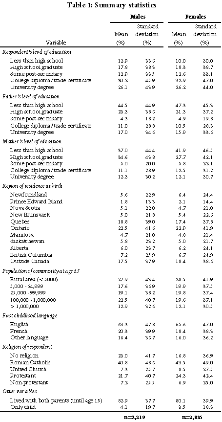
Table 1 presents a complete list of the variables available to us, along with their means and standard deviations. Notice that, with the exception of the education of the respondent at age 30-39, all the information presented in Table 1 would have been available when the individual was a teenager. Thus, if the respondent’s educational attainment is found to be correlated with that information, it may be possible to predict the ultimate education of individuals who are currently in their teens.

Table 1

Statistical Analysis

We subjected the data to a statistical technique known as regression analysis in order to determine which of the socio-economic variables were most closely correlated with educational attainment. We found that only three categories of variables had statistically significant effects. These were: the education of the parents, whether the individual lived with both of his or her parents until age 15, and (to a lesser extent) the population of the community in which the individual lived at age 15. Variables that proved to have no (or little) significant effect on educational attainment were: province of birth (if Canadian), whether the individual was an only child, immigration status, mother language, and religion.

Most importantly, we were able to use the results of our analyses to predict the probability that the respondent would achieve each of the five education levels, based on: parental education, whether the respondent lived with both parents until age 15, and the population of the community in which the respondent lived at age 15.

Parents’ Education

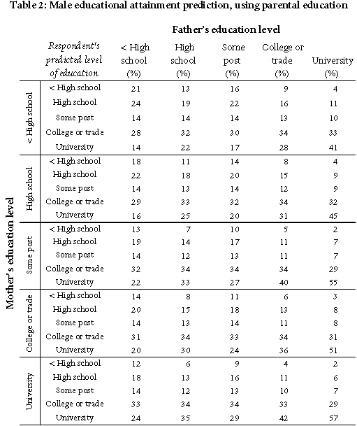
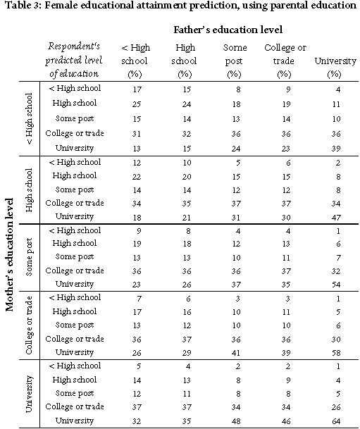
Tables 2 and 3 provide detailed information concerning the impact of parental education on the educational attainment of sons and daughters, respectively. As an example of how to read these tables, the top left box in Table 2 indicates that if both the mother’s and the father’s educations were less than high school (“< High School”), the probability that their son would also obtain less than high school education was 21 percent. The probability that he would finish high school was 24 percent, would finish “some” post-secondary schooling was 14 percent, would finish a trade or college education was 28 percent, and would finish university was 14 percent.

Table 2

Table 2 also indicates that, for males, the probability of completing the two “middle” levels of education – “some university or college” or
“college/trade school” – is not strongly influenced by parental education. For example, the probability of completing college or a trade varies only from 28 percent (when both parents had less than high school or had university) to approximately 34 percent (all other parents); and the probability of completing some college or university varies from 7 percent to 14 percent.

Similarly, Table 3 indicates that, for females, the probability of completing college or a trade varies only from 26 percent (when both parents had university) to 36 percent (most other parents); and the probability of completing some college or university varies from 5 percent to 15 percent (with a much smaller range if university educated parents are omitted).

Table 3

At either end of the educational range, however, parental education is a much more important predictor. When both parents have less than high school, for example, the probability that the child will complete high school or less is 42 percent for females (25 percent high school plus 17 percent less than high school) and is 45 percent for males; whereas when both parents have university educations, these probabilities fall to 5 and 8 percent, respectively.

Conversely, the probability that children will obtain university education rises from 13 percent for females and 14 percent for males, when both parents have less than high school, to 64 percent for females and 57 percent for males, when both parents have university degrees.

Furthermore, a one step change in parents’ education at either end of the educational range can have a dramatic effect on the child’s educational attainment. For example, whereas the probability that males would complete high school or less was 45 percent when their parents both had less than high school, that probability fell to 29 percent when their parents had completed high school.

And whereas the probability that females would complete university was 64 percent when both parents had also completed university, that percentage fell to 39 percent when both parents had college degrees or trade certificates.

Finally, it is important to note that the child’s educational attainment is influenced by the education of both parents. At most levels of education, an increase in the mother’s education has virtually the same effect on the child’s educational attainment as does an increase in the father’s education.

Lived with Both Parents

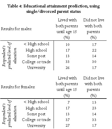
We were also able to use our statistical analyses to predict the effect that living with both parents had on individuals’ educational attainments. These predictions are reported in Table 4. There it is seen that, although living with both parents had a statistically significant effect on the child’s educational achievement, for practical purposes the impact is small. In particular, among both males and females, those who lived with both their parents were approximately 6 percent less likely to drop out of school before completing high school, and 9 percent more likely to complete university, than were those who lived with only one parent.

Table 4

Urban/Rural

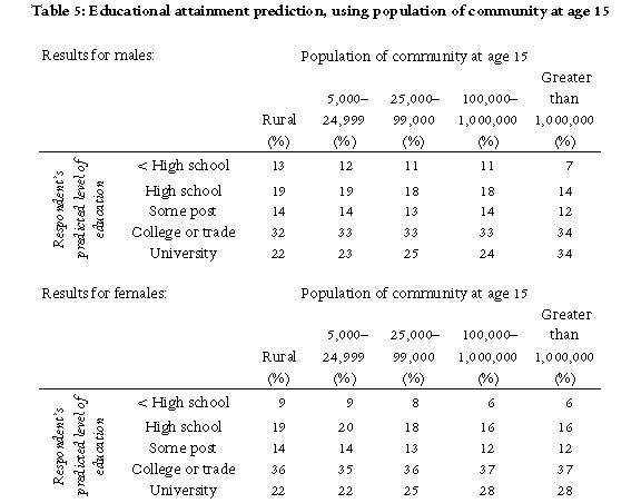
Finally, Table 5 indicates that population of the area of residence makes very little difference to the educational decisions of females and has an important effect on the decisions of males only in very large cities, where males are approximately 10 percent more likely to attend university than are residents of smaller areas.

Table 5

Conclusion

Our results confirm earlier researchers’ findings that, in the prediction of the child’s educational attainment, virtually the only factor that is of importance is the education of the parents. Most importantly, the children of parents with less than high school education are much less likely to proceed beyond high school than are the children of parents at other educational levels. And the children of parents with university degrees are much more likely to complete university themselves than are the children of parents with lesser education.

Nevertheless, we also found that the education levels of the child’s parents were only indicative of a child’s educational attainment. The only situation in which 50 percent of the children of a set of parents had the same educational level as their parents (when both parents had the same education) was that in which both parents had university degrees. In every other case, it was rare for the probability that children would share their parents’ educational attainment to exceed 33 percent. This strongly suggests that, in the prediction of a child’s educational success, experts should generally present at least two (and, more often, three) alternative scenarios.

From 2003 until 2005, Carmen Anderson was a consulting economist at Economica, with a Master of Arts degree from the University of Calgary.

Christopher Bruce is the President of Economica and a Professor of Economics at the University of Calgary. He is also the author of Assessment of Personal Injury Damages (Butterworths, 2004).

Forecasting the Rate of Growth of Real Wages (Productivity)

Posted on March 1, 2004March 24, 2017 By economica

by Christopher Bruce

This article first appeared in the spring 2004 issue of the Expert Witness.

One of the most important determinants of the value of an individual’s lifetime income is the rate
at which that income will grow from one year to the next. The lifetime income of an individual whose earnings grow at 1 percent per year will be dramatically lower than that of an individual whose earnings grow at 5 percent per year. Two major factors determine this growth rate, once the individual has chosen an occupation. First, as workers obtain more experience, their earnings increase due to what is often called
“career progress.” Second, all workers in society tend to benefit equally from the long-term rise in wages across the economy. (If average wages rise by 50 percent over a period two decades, we expect that the wages of labourers and waitresses will increase by 50 percent also, even if the skills required for those two jobs remain unchanged.²)

Furthermore, economy-wide wage increases can be divided into those that are due to changes in the consumer price index – inflationary increases – and those that are due to changes in the “real” purchasing power of wages – real wage increases. (The observed, or “nominal,” rate of increase of wages equals the rate of price inflation plus the rate of increase of real wages.) Unfortunately, despite its importance for the calculation of damages, the forecast of real wage increases proves to be very complex. The purpose of this article will be to report some recent developments in the preparation of that forecast that should prove to be valuable to the courts.

Introduction

Effectively, an increase in the real wage is an increase in the purchasing power of workers’ earnings. But, in the
long run, the average worker will only be able to consume more goods and services if output per worker has increased. Therefore, one would expect there to be a correlation between the long run rate of growth of real wages and the rate of growth of (real) output per worker, or “labour productivity.”

Depending upon the purpose to which it is to be put, a number of different definitions of labour productivity have been proposed. The definition that is most relevant to the determination of real wages is output per hour worked. Changes in this measure are influenced by three factors: increases in the amount of capital goods (machinery, buildings, computers, etc.) per worker, improvements in the technology “embodied” in capital (technological change), and changes in the productivity of workers (usually attributed to improvements in education).

Theory

Because a portion of any change in output per worker is attributable to changes in the quality and quantity of the capital available to workers, some of that increase in output will be paid to the owners of capital. Recently, most economists have come to accept the view that the allocation of gains between capital and labour will be determined in large part by the relative scarcity of those two factors.³ That is, in periods in which labour is in short supply (relative to capital), workers will be able to capture most of the gains from increased productivity and the percentage increase in real wages will equal or exceed the percentage increase in productivity. Conversely, when capital is in short supply relative to labour, it is capital that will capture most of the gains.

One of the attractive features of this theory is that it helps to explain many of the movements in real wages and labour productivity that have been observed over the last five decades. In the 1950s and 1960s, when the economy was growing rapidly and labour was (relatively) in short supply, real wages rose quickly, and at a rate higher than the rate of increase of output per worker. In the 1970s and 1980s, however, when the baby boom generation began to enter the labour market, labour supply increased significantly. Furthermore, because young adults borrow heavily – to purchase homes, cars, furniture, etc. – the influx of young baby boomers drove up interest rates, impeding firms’ ability to borrow for investments in capital. As a result, real wages stagnated even though productivity rose steadily. In the latter half of the 1990s, however, the baby boomers began to approach retirement age. Not only did the supply of labour start to fall, but older workers began to accumulate retirement savings, making funds available for capital investments. The result is that labour has become scarce relative to capital; and economists are now predicting that increases in real wages will begin to match, or exceed, the growth in output per worker.

Empirical evidence

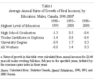
Many economists believe that the reversal in the relative scarcities of labour and capital began in the mid-1990s. Some evidence in support of this conclusion is provided in Table 1. There it is seen that, between 1990 and 1995, the real incomes of Canadian males (25-44 years old, working full-time, full-year) decreased by 0.8 percent per year. (Nominal incomes increased by 1.4 percent per year during that period, while inflation averaged 2.2 percent.) However, between 1995 and 2000, average incomes increased by 3.1 percent while inflation was 1.7 percent, resulting in real income growth of 1.4 percent per year. Table 1 also reports that the real incomes of university graduates grew at 1.7 percent per year in the late 1990s; and that those of high school graduates and holders of trades diplomas and certificates made modest, but positive, gains in that same period.⁴

Table 1

Most Canadian economists appear to believe that, over the long run, output per worker will increase at between 1.5 and 2.0 percent per year. The 2.0 percent forecast is the consensus prediction of a group of Canada’s leading academic and government economists.⁵ The lower predictions have been made by forecasting agencies: Global Insight has forecast 1.9 percent per year over 2002-26; Informetrica has forecast 1.6 percent over the same period; and the Conference Board of Canada has forecast 1.46 percent over 2002-15.⁶Thus, as the model described above suggests that real wages will increase more rapidly than productivity, as the baby boomers age, a conservative estimate would be that real wages will increase by 2 percent per year over the next two decades.

>Conclusion

It is important to note that this means that all workers’ real wages will increase by 2 percent per year. Economy-wide productivity gains are like a rising tide, they carry all workers with them equally. Even the individual who remains in the same job, with no personal increase in productivity and no promotions, can expect, on average, to benefit from real wage increases of 2 percent per year. With inflation predicted also to be 2 percent per year, he or she is predicted to benefit from nominal wage increases of approximately 4 percent per year – a 2 percent inflationary increase plus a 2 percent real increase.

Footnotes:

1. This discussion is taken from Chapter 5 of Christopher Bruce, Assessment of Personal Injury Damages, 4th Edition, Butterworths, 2004.[back to text of article]

2. Evidence that all wages in the economy rise together, regardless of differences in the rate of increase of productivity among industries, was provided by Christopher Bruce in The Connection Between Labour Productivity and Wages (The Expert Witness Vol. 7, No. 2).[back to text of article]

3. See, especially, J. C. Herbert Emery and Ian Rongve, “Much Ado About Nothing? Demographic Bulges, the Productivity Puzzle, and CPP Reform,” Contemporary Economic Policy, 17 January 1999, 68-78; Henning Bohn, “Will social security and Medicare remain viable as the U.S. population is aging?” Carnegie-Rochester Conference Series on Public Policy 50 1999, 1-53; and William Scarth, “Population Aging, Productivity and Living Standards;” in Andrew Sharpe, France St.-Hilaire, and Keith Banting, eds. The Review of Economic Performance and Social Progress 2002, Institute for Research on Public Policy, Montreal, 2002, 145-156.[ back to text of article]

4. U.S. data also suggest that there was a striking switch to a high productivity growth regime in the mid-1990s. See, for example, James Kahn and Robert Rich, “Tracking the New Economy: Using Growth Theory to Detect Changes in Trend Productivity,” Staff Reports, Federal Reserve Bank of New York, No. 159, January 2003.[ back to text of article]

5. Andrew Sharpe,
“Symposium on Future Productivity Growth in Canada: An Introduction,” International Productivity Monitor, 7, Fall 2003, 44-45.[ back to text of article]

6. These figures are taken from Andrew Sharpe, ibid. pp. 44-45.[ back to text of article]

Christopher Bruce is the President of Economica and a Professor of Economics at the University of Calgary. He is also the author of Assessment of Personal Injury Damages (Butterworths, 2004).

Predicting post-secondary education attainment

Posted on June 1, 2003March 24, 2017 By economica

by Mohamed Amery

This article first appeared in the summer 2003 issue of the Expert Witness.

When the plaintiff is a teenager, the first step in predicting that individual’s without-accident earnings capacity is to predict the level of education that would have been achieved by that individual. A recent study, by George Butlin of Statistics Canada, provides a considerable amount of new information concerning the factors that determine whether a high school graduate will enter trade-school, college, or university.

One of the most important of these factors is the education of the parents. Whereas 70 percent of high school graduates with at least one university educated parent attended university, only 43 percent of graduates whose parents had college or trade-vocational level education did so. At the same time, of the graduates whose parents had less than or equal to a high-school education level, only 30 percent participated in university. Conversely, just 18 percent of graduates whose parents were university educated attended a community college.

Butlin also found that, of high-school graduates who failed a grade in elementary school, only 11 percent attended university. This figure is significantly lower than the 46 percent university attendance rate for those who did not fail an elementary grade. He hypothesised that “failing a grade in elementary school may be an indicator of a range of problems beyond academic difficulties [such as] family problems, behavioural problems, psychological problems, language problems, and so forth.” That is, the same factors that resulted in students’ failing elementary grades were also at work in deterring students from entering university.

High-school graduates from two-parent families were found to be more likely to attend university than those from lone-parent households. However, Butlin also found that there were no major differences between two-parent and lone-parent families regarding a graduate’s participation in college or trade-vocational schooling. Those from rural areas were also found to have a lower likelihood of attending university than those from urban areas (34 percent versus 45 percent).

Finally, Butlin found that participation in extra-curricular activities while in high-school acted as a predictor of enrolment at university. High school graduates who had either worked at a job for less than 20 hours per school week throughout their high school years, or who had not worked during their last year of studies at all, had a 45 percent likelihood of attending university. Whereas, of those students who had worked more than 20 hours per week, only 27 percent proceeded onto university schooling. This is not to say that working while in high school “causes” students to choose educational streams other than university. Rather, a more plausible hypothesis is that students who do not intend to enter university take their high school studies less seriously than do those who plan to continue their education and, hence, have more time available for work. Nevertheless, participation in extra-curricular activities can be an important piece of information when predicting the post-secondary education of teenagers.

Reference

Butlin, G. (1999), “Determinants of Postsecondary Participation” 5(3) Education Quarterly Review (Ottawa: Statistics Canada, Catalogue No. 81-003), 9-35.

Mohamed Amery was a research assistant with Economica and an honours economics student at the University of Calgary.

The impact of parental divorce or death on adolescents’ education & earnings

Posted on June 1, 2003March 24, 2017 By economica

by Christopher Bruce
& Mohamed Amery

This article first appeared in the summer 2003 issue of the Expert Witness.

It is sometimes argued that individuals’ earnings will be lower if they grow up in single parent homes than in homes with two parents. If this argument is correct, it is possible that the loss of earnings experienced by a child who has been injured will be lower if that child came from a one-parent family than from a two-parent family. Conversely, however, the loss suffered by a child whose parent has been killed may be higher than would normally be assumed if the loss of that parent has meant that the child must now grow up in a single-parent family.

A number of studies are available that have explored the effect of parental absence due to divorce or death on adolescents’ labour market outcomes as adults. Although these studies are consistent in finding that the absence of a parent has some effect on adult earnings, they disagree on what that effect is. Corak, for example, concluded that whereas the earnings of women were the same regardless of family backgrounds, those of men from divorced families were approximately three percent lower than those of men from intact families.

Lang and Zagorsky confirmed Corak’s finding that “parental presence early in life [has only a minor effect on] economic well-being in adulthood” (p. 255). Nevertheless, whereas they found that a father’s presence is important for the educational attainment of both sons and daughters, a mother’s presence is significant only for the educational attainment of daughters. Also, contrary to Corak, they found (p. 255) a “strong impact of father’s presence on [a] son’s probability of being married”.

Fronstin et. al. concluded that the wages of “females, but not males, appear to be adversely affected by a father’s death, particularly when the death occurs before the child’s sixteenth birthday” (p. 151). The primary impact on men was higher unemployment rates (at age
33), particularly if the father had died when the son was between 16 and 22. Fronstin et. al. also found that disruptions occurring prior to “middle teenage years have somewhat greater adverse effects on educational attainment, while disruptions occurring into young adulthood have [their primary] adverse effects on … labour market outcomes” (p.
168).

In their book, Growing Up with a Single Parent, Sara McLanahan and Gary Sandefur, summarized the findings of a number of studies that had been conducted in the 1980s. Those studies generally found that children who were raised in single-parent families were somewhat less likely to attend college than were children of two-parent families, and much less likely to graduate from college. However, there was clear evidence that these effects were much less severe if one parent had died than if the child’s parents had divorced or had never married. These results suggest that it is not “single-parenting” per se that yields adverse effects. Rather, single parenting appears to act as a proxy for the underlying factors that lead parents not to marry, or to divorce. It is those unobserved factors that appear to have the primary impact on children’s labour market success.

Finally, Boggess found that living with a widowed, divorced, or separated mother had no effect on educational attainment. Interestingly, however, he concluded that “living in a stepfather family appears to have a persistent negative effect on high school graduation rates” (p. 205).

What these studies appear to suggest is that a child from a single-parent family may obtain slightly less education, and perform slightly less well in the labour market, than a child from a two-parent family. However, this effect will be much more pronounced if the child’s parents had never married or had divorced than if one of the child’s parents had died.

References

Boggess, S. (1998) “Family Structure, economic status, and Educational Attainment” 11(9) Journal of Population Economics,
205–222.

Corak, Miles (2001), “Death and Divorce: The Long-term Consequences of Parental Loss on Adolescents” 19(3) Journal of Labor Economics,
682-715.

Fronstin, P. et al. (2001) “Parental Disruption and the Labour Market Performance of Children When they Reach Adulthood” 14(4) Journal of Population Economics, 137 – 172.

Lang, K. and J. L. Zagorsky (2000) “Does Growing Up With a Parent Absent Really Hurt?” 36(2) The Journal of Human Resources, 253-272.

McLanahan, S., and G. Sandefur, Growing up with a Single Parent (Cambridge, Mass.: Harvard University Press), 1994.

Christopher Bruce is the President of Economica and a Professor of Economics at the University of Calgary. He is also the author of Assessment of Personal Injury Damages (Butterworths, 2004).

Mohamed Amery was a research assistant with Economica and an honours economics student at the University of Calgary.

The Connection between Labour Productivity and Wages

Posted on June 1, 2002March 24, 2017 By economica

by Christopher Bruce

This article first appeared in the summer/autumn 2002 issue of the Expert Witness.

Many readers of this newsletter will have received personal injury damage assessments in which the expert has argued that wages in a particular industry will increase at some rate – for example, 1.5 percent per year – “because” output per worker (productivity) in that industry is projected to increase at that rate.

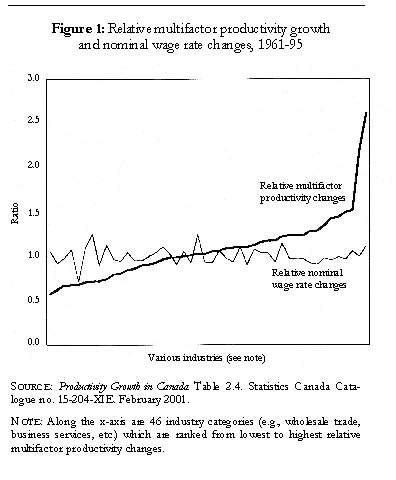
What I wish to show in this article is that, as appealing as this argument may be to the layperson, it is wrong. Not only does economic theory predict that the connection between industry productivity and wages in that industry will be tenuous at best; empirical evidence reveals that there has been virtually no connection whatsoever between industry wages and industry productivity in Canada.

I proceed by first describing the method that agencies like Statistics Canada use to measure labour productivity. I then describe the economic theory of how wages are determined within industries and occupations. In a third section, I contrast that theory with the theory of national wage determination. Finally, I present some recent statistical data concerning the relationship between the rate of growth of productivity and the rate of growth of wages at the industry level in Canada.

Measurement

Statistics Canada obtains an index of the “real”
level of output in each industry by dividing the total revenues received by the firms in that industry by an index of the industry’s prices. For example, if total revenue in the clothing industry was $100 billion in 2001 and the clothing retail price index was 125, the index of real output would have been calculated to be 800 million. If revenues rose to $110.5 billion in 2002 and the price index rose to 130, the output index would have risen to 850 (million).

Labour productivity, or output per hour of work, is then found by dividing the (real) output index by the number of hours worked by individuals in that industry. If clothing workers worked 100 million hours in both 2001 and 2002, for example, output per worker hour would be found to have increased from 8.00 to 8.50 between those years, or by 6.25 percent.

Note that there is no connection between revenues per worker and output per worker. It is quite possible, for example, for revenue to rise because prices have risen while labour productivity has remained unchanged. Conversely, even if output per worker has risen substantially, if prices have fallen revenue per worker may have remained constant or even fallen.

Theory – Industry Wage Levels

Those who believe that there is a connection between labour productivity and wages within an industry (or occupation) implicitly assume the following: When output per worker increases, workers’ contributions to firm revenue increase causing demand for workers to increase also. As wages are determined by supply and demand, an increase in demand will imply an increase in wages.

This “theory” is wrong for two reasons. First, there is no necessary connection between output per worker and revenue per worker. As was pointed out above, if demand for the industry’s product is decreasing, the price that can be charged for that product will also be decreasing. Hence, even if output per worker rises, revenue per worker may fall.

Furthermore, when output per worker increases, the industry will have to sell additional units of output; that is, industry supply will rise. But, by the laws of supply and demand, when supply increases, prices decrease. That is, the increase in worker productivity may cause a decrease in prices.

In some cases, this decrease in prices is so extreme that an increase in worker productivity may actually cause a decrease in revenue per worker. The clearest example of this phenomenon has occurred in agriculture, where farm incomes are under constant downward pressure even though productivity gains have been greater in that sector than in most other industries.

Second, even if an increase in labour productivity does lead to an increase in revenues generated per worker, it is not necessarily the case that the consequent increase in demand will be associated with a long run increase in wages (relative to other industries). The reason for this is that, in the long run, additional workers can be supplied to that industry, which offsets the upward pressure on wages. That is, when demand for an industry’s workers increases, wages in that industry do not rise relative to wages in other industries. Rather, it is employment in the high productivity industry that will rise relative to employment in other industries.

Assume, for example, that there is a large group of workers who would be approximately indifferent between working as plumbers, carpenters, and electricians. Assume also that, initially, all three receive the same wage rate. Now, if productivity rises among electricians, there will be an increase in demand for electricians. In the short run, say a year or two, it will not be possible to train additional electricians and wages may be bid up.

But, when wages are higher among electricians than among plumbers and carpenters, students graduating from high school will prefer to train as electricians. Soon, the supply of new electricians will increase and the supply of new carpenters and plumbers will decrease. Wages will fall among electricians and will rise among plumbers and carpenters.

Ultimately, the wages of all three occupations will equalize. All three will enjoy higher wages than they did initially. But, among plumbers and carpenters this will have occurred without any increase in productivity. And, among electricians, the wage increase will have been much smaller than the productivity increase, because the effect of that increase will have been diluted by the influx of workers from other occupations.

Indeed, if the initial number of electricians had been considerably smaller than the number of plumbers and carpenters, it is possible that the wage increase experienced by all three groups would have been negligible. The number of workers who would have to leave the plumbing and carpentry trades would have been so small, relative to the total numbers in those trades, that their exit would have had very little effect on wages in those occupations.

The primary effect of the productivity increase among electricians is that the number of electricians will increase and the numbers of plumbers and carpenters will decrease.

Similar effects can be seen in other industries. We know, for example, that in the last 50 years there have been far greater productivity gains in “fast food” restaurants than in restaurants serving “classic cuisine.” Yet, wages have not increased in the former relative to the latter. The primary reason is that every increase in demand for fast food workers has been met by an influx of workers from other unskilled industries.

This is not to say that there is no connection between productivity and wages at the industry level. If the number of workers in an industry is not responsive to changes in wages, an increase in productivity may produce a permanent wage increase. There may, for example, be institutional barriers preventing additional workers from entering an industry – such as union regulations or restrictions on the numbers of students training for that industry at university or college. Alternatively, there may simply be a limited number of individuals who have the aptitude to enter certain industries or occupations. Once that number had been exhausted, further wage increases might not call forth additional labour supply.

Theory – National Wage Levels

Even if there is only a limited connection between wages and productivity at the industry level, there may still be a strong connection at the national level. When productivity gains drive up wages in one industry or occupation, it is anticipated that workers will be drawn from other industries and occupations, thereby returning relative wages to their initial level. If productivity increases at the
national level, however, the equivalent effect would require that workers be drawn from other countries. But, as Canada restricts the number of immigrants, this effect will be much less important for national wage levels than it was for industry wage levels.

Also, a productivity gain at the national level is less likely to lead to a reduction in output prices than is an equivalent gain at the industry level. When output increases in an industry, everything else being constant, the industry may have to lower prices in order to sell that increase. When output increases in the nation as a whole, however, all workers will have higher incomes and those incomes may be used to purchase the increased output. In a sense, the increased output “creates” the increased demand to purchase that output. Prices need not fall.

And if prices do fall, the “real” incomes of all workers will increase. That is, even if observed (or nominal) wages do not change, workers will be able to buy more goods and services with their incomes. They will be better off in a “real” sense. Thus, an economy-wide increase in productivity could cause an increase in the welfare of workers, not through an increase in observed money wages, but through a decrease in average prices.

Evidence

The evidence concerning the connection between industry-level wages and productivity is clear. In its recent publication, Productivity Growth in Canada, Statistics Canada provided information concerning relative productivity growth and relative changes in wages for 46 Canadian industries, from 1961-1995.

These statistics have been plotted in the figure below, with industries ranked from lowest to highest productivity growth over that period. It is seen clearly in that figure that there is virtually no correlation at all between an industry’s relative productivity growth and its growth in relative wages. Indeed, regardless of an industry’s growth in productivity, its relative wages remained unchanged.

Conclusion

There are sound theoretical reasons for predicting that there will be very little correlation between an industry’s productivity growth and its wage growth. The empirical evidence provides strong support for this prediction. Indeed, that support is so strong that it is incumbent on any expert who would argue that a correlation exists between productivity and wages to justify that argument.

Christopher Bruce is the President of Economica and a Professor of Economics at the University of Calgary. He is also the author of Assessment of Personal Injury Damages (Butterworths, 2004).

Combining Occupational Options

Posted on June 1, 2000March 24, 2017 By economica

by Christopher Bruce

This article was originally published in the Summer 2000 issue of the Expert Witness.

In many cases it is not clear at the time of trial what occupation the plaintiff would have entered had he or she not been injured, or what occupation he/she will now enter. In these cases, it is common for the vocational expert to offer a menu of possible occupations that are consistent with the plaintiff’s observed interests and aptitudes.

An issue that is crucial to the correct evaluation of damages in such cases, but which rarely receives the attention it deserves is: How should the incomes from the various occupations be “weighted” to determine an average, expected income for the plaintiff?

For example, assume that the vocational expert has concluded that, with appropriate upgrading, the plaintiff has the aptitude and skills to enter any one of three occupations – A, B, or C. Assume also that the following information is available about these occupations:

Annual incomes are:

A – $20,000
B – $25,000
C – $30,000

The number of employed workers in these occupations is:

A – 5,000
B – 1,000
C – 100

The unemployment rates in these occupations are:

A – 20%
B – 8%
C – 2%

The question is, how should the plaintiff’s expected income be calculated? I can think of four methods, each of which can easily be defended.

Simple Average

If the court has been provided with no information concerning which of these occupations the plaintiff will enter, it can be argued that, ex ante, there is an equal probability that he will enter each of them. Hence, each income should be weighted equally, producing an average of

($20,000 + $25,000 + $30,000)/3 = $25,000

Weight by Employment Opportunities

If it is assumed that the plaintiff will apply at random for jobs advertised in the newspaper, it is more likely that he will randomly “select” occupation A, with 5,000 jobs, than occupation B, with 1,000.

Alternatively, when the individual’s preferences are unknown, it can be argued that he is most likely to enter the occupations that other people have been observed to enter. Thus, as “most” individuals choose occupation A, it can be argued that it is more likely that the plaintiff will choose A than any other, all else being equal.

Recognising that there are 6,100 jobs in total, if income is weighted by employment opportunities, the average proves to be

[(5,000 x $20,000) + (1,000 x $25,000) + (100 x $30,000)]/6,100 = $20,984

Weight by Supply and Demand (Unemployment Rate)

If it is assumed that the plaintiff is more likely to be successful applying for jobs in which there are few applicants relative to the number of positions available, he is more likely to obtain a job at the occupations with the lowest unemployment rates. One method of allowing for this possibility is to weight the annual incomes by the inverse of their respective unemployment rates (that is by 1 minus the unemployment rate). These values are 80% for A, 92% for B, and 98% for C, with an average of 90%. Thus, relative to the average, the plaintiff is assumed to have a 0.889 (80/90) probability of finding a job at A, a 1.022 (92/90) probability of finding a job at B, and a 1.089 (98/90) probability of finding a job at C. In this case, the weighted average of the incomes in A, B, and C proves to be

(0.889 x $20,000 + 1.022 x $25,000 + 1.089 x $30,000)/3 = $25,333

Weight by Income

If it is assumed that the plaintiff is most likely to apply to the occupation with the highest income, the weightings change again. For example, if the probability that the individual will apply to each occupation is strictly proportional to the income earned in that occupation, the probability that he will apply to A is 80 percent of the probability that he will apply to B; and the probability that he will apply to C is 120 percent of the probability that he will apply to B. In this situation, the weighted average income will be

[(0.8 x $20,000) + (1.0 x $25,000) + (1.2 x $30,000)]/3 = $25,667

In the table below, I provide an example of these calculations drawn from a case in which Economica was involved recently. There it is seen that the vocational expert recommended eight possible occupations for the plaintiff. The average incomes for these occupations vary from $36,005 to $40,615, a difference of $4,610 per year, depending on which of the four averaging techniques is applied. If we assume that this individual was 25 years old at the time of the trial, an annual difference of $4,610 will alter the lifetime loss by approximately $100,000.

Clearly, it could prove crucial to determine which method is most appropriate. The first step is to speak to the vocational expert. Only if that expert indicated that the plaintiff was equally likely to enter each of the specified occupations would I consider it appropriate to employ the simple average method. If the expert has no opinion, my preference would be to weight the occupational incomes either by unemployment rate (to reflect supply and demand) or by numbers of employees (to reflect the likelihood that a plaintiff of known characteristics will choose a particular occupation). Weighting by income would only seem to be reasonable if the plaintiff was known to be particularly strongly motivated by financial considerations.

Table 1

Christopher Bruce is the President of Economica and a Professor of Economics at the University of Calgary. He is also the author of Assessment of Personal Injury Damages (Butterworths, 2004).

The MacCabe Judgment: Allowing the Use of Earnings Statistics for Males When Estimating the Future Income of a Female

Posted on September 1, 1998March 24, 2017 By economica

by Derek Aldridge

This article was originally published in the autumn 1998 issue of the Expert Witness.

On October 5, the Alberta court released its decision in the case of MacCabe v. Westlock RCSSD #110 et al (action: 9303 05787). The judgment is important for many reasons, though the most important aspect from an economist’s point-of-view is that it recommended the use of male earnings statistics to estimate the future earnings potential of a female. In particular, it was found that Ms. MacCabe would have followed a career path similar to that of the average male. That is, the court concluded that she would not have taken significant amounts of time out of the workforce for child rearing, and she would not have worked part-time. Therefore, it found that earnings statistics for males should be used to predict what her income would have been.

Some of the most important sections from the decision (related to the male/female income statistics issue) are reproduced here:

[para468] Clearly the evidence establishes that the exceptional individual characteristics of the Plaintiff are such that her abilities would have commanded the equivalent salary of her male counterparts. She would have established a strong attachment to her career. The use of male wage tables is justified. In any event, I am of the view that any award which I grant to the Plaintiff should not and cannot be solely determined by her gender.

[para469] It is entirely inappropriate that any assessment I make continues to reflect historic wage inequities. I cannot agree more with Chief Justice McEachern . . . in Tucker, supra, that the
courts must ensure as much as possible that the appropriate weight be given to societal trends in the labour market in order that the future loss of income properly reflects future circumstances. Where we differ is that I will not sanction the “reality” of pay inequity. The societal trend is and must embrace pay equity given our fundamental right to equality which is entrenched in the constitution. . . .

[para470] . . . The Court cannot
sanction future forecasting if it perpetuates the historic wage disparity between men and women. Accordingly, if there is a disparity between the male and female statistics in the employment category I have determined for the Plaintiff the male statistics shall be used, subject to the relevant contingencies. . . .

[para481] I agree with Dr. Bruce that absent
the accident, the Plaintiff would have been committed to her career and there would not have been a significant withdrawal from the labour force. . . .

So what does this imply about future cases involving injured or deceased females? It seems clear to us that if it is accepted that a young female would have followed a career path similar to that of the average male (in which she works full-time and does not take significant amounts of time out of the workforce for child rearing), then it follows that income statistics for males should be used to estimate her pre-accident income. (We discussed this issue in the Autumn 1997 issue of the Expert Witness.)

But what if it is found that a young woman would have followed a traditional female career path? In this case we suggest that using income statistics for females will still probably underestimate the true income path, but using those statistics for males will probably overestimate the true income. The reality likely lies somewhere in between the two alternatives. However, the MacCabe judgment appears to leave open the possibility that earnings statistics for males could be used even for female plaintiffs who would have followed “traditional” female career paths. It may be the case that the courts will choose to apply earnings statistics for males, regardless of the evidence about the woman’s likely career path – as a sort of “social justice” choice (Recall paragraph 469 of MacCabe: “I will not sanction the ‘reality’ of pay inequity.”)

However, the same argument could possibly apply to other situations in which a certain group of people earn less, on average, than the average male. For example, it is well-known that, on average, Natives earn less than non-Natives. From the MacCabe decision it may follow that one should use average income statistics for males to estimate the potential income of a young Native male (or female), with no adjustment to account for the reality that the average Native earns less than average non-Native. Conversely, perhaps the defense could argue that a person who has been disfigured in an accident should not be compensated for the “appearance-discrimination” component of his loss of income because that would be an endorsement of the “reality” of discrimination. If the court chooses to correct for the reality of pay inequity, then this could raise some difficult issues for those of us involved in loss of income cases.

Derek Aldridge is a consultant with Economica and has a Master of Arts degree (in economics) from the University of Victoria.

Using Industry Growth Rates to Update Census Occupational Earnings Figures

Posted on September 1, 1998March 24, 2017 By economica

by Kris Aksomitis

This article was originally published in the autumn 1998 issue of the Expert Witness.

The most reliable source of information about the incomes of specific occupations is the census. Unfortunately, census data are collected only once every five years — and income data are not published until three years after they are collected. (For example, income data from the 1995 census were not available until July of 1998.)

As a result, if census data are to be used, some method must be found for updating those data between the most recent census year and the year in which the information is required. For example, to use census income data in early 1998 (before the release of the 1995 census data), estimates of 1998 earnings had to be based on data from the 1990 census. This updating is achieved by increasing the relevant census figure by an estimate of the percentage increase in earnings between the most recent census year and the year in question.

The data series which is most often used to obtain this estimate is Statistics Canada’s Annual Estimates of Employment, Earnings and Hours (Cat. 72F0002XDE). This series reports estimates of average weekly earnings by
industry. Hence, as the desired figure is income by
occupation there is some concern that growth rates based on the Statistics Canada occupational earnings series will fail to provide an accurate estimate of the desired increase.

To my knowledge, no one has attempted to test whether industry growth rates provide an accurate estimate of occupational growth rates. That is the purpose of this article.

Here, I calculate the growth rates of incomes in various
occupations between the 1990 and 1995 censuses and compare those growth rates to estimates of those rates, which have been obtained from the annual growth rates of
industry earnings.

Methodology

The purpose of the article is to test the accuracy of using industry growth rates to predict average earnings for specific occupations. As such, the procedure uses the following steps:

First, a number of occupations were selected as a basis of comparison. The selection process was fairly arbitrary, but an attempt was made to include occupations from a number of distinct industries.
Second, data were collected for the chosen
occupations from the 1990 Census and the 1995 Census. These figures represent the actual annual average incomes for these occupations in the respective years. The ratio of the incomes in 1995 and 1990 were calculated for each occupation.
Third, data were collected on industry income growth rates. These figures were calculated from average weekly earnings for the specific industries in question, and were used as proxies for salary growth rates within those industries.
[Note that the calculated figures for both industry and occupation are simple percentages and not compound growth rates. For example, the calculated “all occupations” growth factor of 13% means that earnings increased 13% in total over the 5 years, or slightly less than 2.5% compounded annually. For each industry or occupation, the growth factor was calculated by dividing the value of 1995 earnings by the value of 1990 earnings.]
Fourth, the “actual” rate of growth of earnings for each occupation was compared to the growth rate of earnings from the industry that I believed to be most closely related to the occupation in question. In the table, below, I refer to these industry growth rates as “estimated” rates of growth as they represent our best estimates of the growth of occupational earnings.
Finally, the actual occupational growth rates were compared with both the estimated growth rates and the average, “all-industry” growth rate.

Analysis

The table presents the results. A number of interesting observations can be drawn from the data. The first, and most important observation, is that the industry specific growth rates provide a better estimate than the overall average growth rate in all but five cases.

From this observation, it can be argued that, for the most part, the industry-specific estimated growth rates provide a better estimate of earnings growth than do the average growth rates for the entire economy. Of the occupations I examined, only for male food service supervisors did the average growth rate provide a significantly better estimate than did industry-specific growth.

A second observation is that the estimates provided by the industry specific growth factor is quite accurate in the majority of the cases. For example, in 12 of the 22 cases, the estimated earnings are within 5.1% of the actual earnings. This indicates that, in these cases, the annual compound growth rate predicted by the estimate is within 1% of the actual annual growth rate in earnings.

Some of the errors can be explained by the small sample size of the occupations. This would appear to be the case, for example, with respect to female petroleum drillers. In other cases, for example male bookkeepers, it may be that individuals were spread among so many industries that no estimate from a single industry could be expected to prove accurate.
[Interestingly male bookkeepers and female drillers were the only two occupations of those I’ve examined whose
earnings were lower in 1995 than in 1990. In every other case, actual earnings increased over the 5-year Census period and the earnings estimates by the model provided a reasonable estimate of actual earnings.]

A final observation from the data is that the correlation between actual and predicted earnings seems highest in occupations which are characterised by a high degree of unionization. For example, accurate estimates were obtained for police, social workers, registered nurses and railway workers.

Conclusions

Overall, it seems that industry-specific growth rates provide a reasonable estimation of occupational growth. In the majority of cases, the specific industry growth rate provided a better estimation of actual earnings growth than did the general economy growth rate. Further, in many cases the industry wage growth rate provided an excellent proxy for the specific occupational growth rate, especially in those occupations that were most highly unionized and clearly defined as part of that industry.

Kris Aksomitis was a research associate with Economica Ltd. and an MA student in Economics at the University of Calgary.

The Effect of Alcoholism on Earning Capacity

Posted on June 1, 1998March 24, 2017 By economica

by Nicole MacPherson

This article was originally published in the summer 1998 issue of the Expert Witness.

It seems common sense to argue that alcoholics will experience reduced earning capacity. Thus, all else being equal, alcoholics will be eligible for lower damage awards than will other plaintiffs. What is often not clear, however, is how severe the effects of alcoholism will be.

The purpose of this article is to summarise the statistical literature concerning the effects of alcohol consumption on earnings and employment. One of the most important findings of this literature is that alcoholism has both direct and indirect effects on earnings. That is, there is evidence that alcoholics’ earnings are depressed both because alcoholism causes reduced labour productivity and because it discourages investments in “human capital” (e.g., education). Problem drinking is also found to increase unemployment.

Direct Effects

Alcoholism is considered to be a disease, and affects earnings as such. The physical and mental health problems associated with problem drinking have direct effects on labour market productivity and reliability. That is, sickness, hangover, late arrivals, extended lunch breaks, and early departures are some work characteristics that lead to reduced reliability and productivity. This in turn leads to lessened earnings and fewer promotions and raises.

Alcoholism can have other direct effects on wages, namely, alcoholism can affect career choices and stability. It is possible that alcoholics self-select into jobs that are less demanding, and therefore lower paying. The further advanced the state of alcoholism, the less the alcoholic is concerned about his or her career. Therefore, alcoholics tend to gravitate towards jobs that are not strenuous or taxing.

Indirect Effects

An important way in which alcoholism can affect earnings is through its effect on human capital characteristics. If the disease is advanced in youth, the alcoholic may not have the stamina to complete schooling, post-secondary or otherwise. This possible lack of education could lead to lower wages and selection into “dead-end” jobs. It is important to note that alcoholics may select into such jobs because of choice (the direct effect) or because of a lack of education (the indirect effect).

It is likely that alcoholics will have difficulties maintaining employment due to their condition. The reduced reliability discussed above can lead to job losses and decreased employability. The subsequent lack of work experience can lead to lower wages and earnings.

A significant indirect effect arises from familial and relationship problems associated with alcoholism. Alcoholics have higher divorce rates than non-alcoholics. As well, there is a higher probability of an abusive home life among problem drinkers. The emotional and mental strains arising from these factors can be expected to have negative impacts on productivity, and therefore earnings.

Empirical Evidence

Alcoholism’s effect on earnings has been the subject of a number of recent scholarly articles, which attempt to estimate this impact empirically. These studies indicate that, when direct and indirect effects are combined, alcoholics earn approximately 40 percent less than non-alcoholics. When human capital characteristics are controlled for, alcoholism alone leads to an 18 percent reduction in wages. That is, almost one half of the effect of alcoholism on earnings is due to lower human capital characteristics, namely education and work experience. Conversely, this implies that an alcoholic will earn approximately 18 percent less than will others with similar education levels and work histories.

It is significant to note that alcoholics earn less not only because of the effect heavy drinking has on human capital, but also because of the nature of alcoholism. A recent study found that alcoholics are more likely to be unemployed than alcoholics, and earn less when they are employed, even after controlling for the effect of education and experience. As the disease progresses, the earnings potential of the alcoholic lessens.

Alcoholism and employment have a causal relationship. Alcohol abuse negatively affects employment, but lack of work also affects drinking habits. Depression and stress resulting from unemployment can lead to increased reliance on alcohol and other drugs. Alcoholics can enter a vicious circle in that the longer an individual is unemployed, the more advanced the state of alcoholism. As the disease becomes more debilitating, becoming employed is increasingly difficult.

Recent medical research has found that moderate alcohol use leads to health benefits such as reduced risk of cardiovascular disease. Since healthy employees are productive employees, it is not unreasonable to suggest that moderate drinking can lead to greater productivity, and therefore higher earnings. In fact, there is evidence to support the hypothesis that alcohol and earnings have a parabolic relationship. That is, teetotalers and heavy drinkers both earn less than moderate drinkers. In fact, studies show that non-drinkers earn between eight and ten percent less than moderate drinkers. It has been estimated that wages peak for individuals consuming an average of 2.40 drinks per day, which is consistent with the medical literature. Individuals who do not drink at all may miss out on the health benefits of moderate drinking, as well as on social opportunities and networking to further their careers. Conversely, alcoholism deteriorates one’s state of health. As well, alcoholics may endure public shame because of their condition, and this can decrease the opportunities to advance their careers at social functions.

It is vital to realize that a future alcoholic may currently display only minor symptoms of problem drinking. Alcoholism is a disease, and when left untreated can have ravaging effects on the individual’s physical and mental states. These effects can have significant negative impacts on employment, productivity, and earnings.

The lost productivity and lowered earnings of alcoholics are significant costs that have merited recent attention in the economic literature. The alcoholic and his or her family suffers from lowered earnings. Employers and co-workers suffer from the alcoholic’s lost productivity. In addition to the well-known costs of alcoholism, illnesses, automobile accidents, and crime, problem drinking leads to decreased productivity and therefore, lower wages and earnings.

References

Berger, M.C., and Leigh, J.P. “The effect of alcohol use on wages”, Applied Economics, 1988, 20, 1343-51.

—. “Schooling, Self-Selection, and Health”, Journal of Human Resources, 1989, 24 (3), 433-455.

Boffetta, P., and Garfinkel, L. “Alcohol drinking and mortality among men enrolled in an American Cancer Society prospective study”, Epidemiology, 1990, 1, 342-348.

French, M.T., and Zarkin, G.A. “Is moderate alcohol use related to wages? Evidence from four worksites”, Journal of Health Economics, 1995, 14, 319-344.

Hamilton, V., and Hamilton, B. “Alcohol and earnings: Does drinking yield a wage premium?”, Canadian Journal of Economics, 1997, 30 (1), 135-151.

Kenkel, D.S. “Health Behaviour, Health Knowledge, and Schooling”, Journal of Political Economy, 1991, 99 (2), 287-305.

Mullahy, J., and Sindelar, J. “Gender Differences in Labor Market Effects of Alcoholism”, American Economic Review 1991, 81 (Papers and Proceedings), 161-165.

— “Alcoholism, Work, and Income”, Journal of Labor Economics, 1993, 11 (3), 494-520.

— “Employment, unemployment, and problem drinking”, Journal of Health Economics, 1996, 15, 409-434.

Shahaheh, B. “Drug and alcohol abuse in the workplace: Consequences and countermeasures”, International Labour Review, 1985, 124 (2), 207-223.

Zarkin, et. al., “Alcohol use and wages: new results from the National Household Survey on Drug Abuse”, Journal of Health Economics, 1998, 17, 53-58.

Nicole MacPherson was a Master of Arts student at the University of Calgary. She wrote a thesis on the topic of “Alcohol, Gender, and Labour Market Outcomes.”

Economic and Employment Prospects of the Disabled

Posted on June 1, 1997March 24, 2017 By economica

by Therese Brown

This article first appeared in the summer 1997 issue of the Expert Witness.

Most research concerning the effects of disability on earnings and employment uses cross-sectional data — that is, data which are collected for a large group of individuals at one time. The impact which an injury incurred this year will have in ten years time is inferred by comparing the status of individuals who have recently been injured with the equivalent status of those who incurred their injuries ten years ago.

This approach suffers from two serious drawbacks. First,
those who are injured today may differ in many significant ways from those who were injured ten years ago. Second, it is difficult to use cross-sectional data to determine the “life courses” of individuals. For example, assume that it has been observed that the unemployment rate of those who suffered a particular type of injury in the past is consistently 20 percent regardless of how many intervening years have passed. Does that mean that 20 percent of those with that type of injury have been unemployed for 100 percent of the time? That
100 percent of the individuals have each been unemployed for 20 percent of each year? Or some position in between?

One possible way of dealing with these problems would be to rely on panel data — that is, data from studies
which “follow” individuals for a number of years. For example, some of the issues identified above could be resolved if disabled individuals could be followed for a number of years after their accidents had occurred.

One study which uses this type of data (from the United States) is “Employment and Economic Well-Being Following the Onset of a Disability” by Richard Burkhauser and Mary Daly. In the interests of providing an all-encompassing perspective, the authors define disability in a broad sense, allowing them to include individuals who have been integrated into the workforce. Further, their analysis considers only those who report a physical or nervous condition that has limited their work capability for at least two consecutive years.

The authors estimate the prevalence of disability among individuals between the ages of 25 and 61 — prime working ages — to be 9.2 percent for males and 10.6 percent for females. Results from their multi-period analysis of these individuals suggest that the onset of disability is not accompanied by a dramatic reduction in economic well-being
(especially once government income is included) — a considerably different finding from that reported by other studies utilising cross-sectional data.

Particularly interesting for our purposes are their estimations of the cumulative risk that disabled persons will experience particular events. Their sample population is aggregated into a younger group of 25 to 50 year olds and an older group of 51 to 61 year olds. Their results indicate that
15 percent of the younger group and 24 percent of the older group had stopped working for at least one full year, one year after experiencing the disabling condition. After five years,
44 percent and 53 percent of the younger and older group, respectively, had experienced at least one year of no work. For those in the younger group who stopped working for a year, many subsequently returned to work. After one year, 28 percent of this group had returned to work, and by five years the majority
(61 percent) had returned to work. Fewer of the older group had resumed employment, with only 14 percent after one year and 28 percent after five years. In terms of economic well-being, in both the younger and older groups, 46 percent earned an income that was at least equivalent to their pre-accident income after one year, with the majority reaching their pre-disability income after 2 years. At a five-year point following the onset of the disability, 84 percent in the younger group and 75 percent in the older group had returned to a level of household income that was at least equivalent to their pre-onset income.

The authors point out that poverty is not unknown to many people who report disabling experiences, as within a five year period 22 percent of this population had fallen into poverty for at least one year. They suggest, however, that the loss of income experienced by disabled individuals is less notable on average than might be expected. Their analysis also suggests that older workers are likely to be more negatively affected by their disabling condition than are their younger counterparts, in terms of reintegration into the workforce and restoration to their pre-onset economic position. The authors indicate that government transfer payments have a larger role in the income recovery of disabled individuals than does the recovery of their health, as the experience of health recovery is relatively rare. They also conclude that there is a longer time period than was previously expected between the time that an individual becomes disabled and the time they exit from the labour market or enter the disability or retirement rolls.

From 1996 through February 1998, Therese Brown was a consultant at Economica.

The Children of Immigrants – How Do They Fare?

Posted on June 1, 1997March 24, 2017 By economica

by Therese Brown

This article first appeared in the summer 1997 issue of the Expert Witness.

It has been argued that one of the factors relevant in predicting the income of minors is the immigrant status of their parents. In this vein, it has been suggested that those with foreign-born parents will not do as well as those with Canadian-born parents. This assumption is based on the belief that the former have a disadvantage deriving from a lack of familiarity with the culture, labour market institutions, and in many cases with the language. Our research does not support this theory. There is considerable evidence, rather, to suggest that second generation Canadians will surpass their more established counterparts.

The Socio-economic Indicators of Success

Numerous studies have lent support to the view that those with foreign parentage are not disadvantaged by that fact, either in terms of earnings, or educational and occupational attainment. A study by Charles M. Beach and Ross Finnie, “A Recursive Earnings-Generation Model For Canadian Males,” found the effect on earnings of having grown up with immigrant parents to be positive, and substantially so. Barry Chiswick and Paul Miller found in their study “Earnings in Canada: The Roles of Immigrant Generation, French Ethnicity, and Language,” that men who have at least one foreign-born parent earn 13 percent more than comparable men with native-born parents. Even if all else is held constant, Canadian-born sons of immigrants have earnings which are two percent higher than their male counterparts with native-born parents. What Chiswick and Miller found particularly striking was the consistency with the findings of other studies in Canada, the U.S. and Australia. This would suggest that American studies are relevant in this discussion as well.

In an American study entitled, “Sons of Immigrants: Are They at an Earnings Disadvantage?” Barry Chiswick states that sons with one or more foreign-born parents have higher earnings on average than those with native-born parents, if other things are held constant. The earnings advantage is approximately eight percent, four percent, and six percent respectively for those who have a foreign-born father, a foreign-born mother, or two foreign-born parents. Another American study undertaken by Geoffrey Carliner, “Wages, Earnings and Hours of First, Second, And Third Generation American Males,” showed that second generation males had higher wages and earnings, in addition to working more hours, than did their third generation counterparts.

Advantages accruing to the second generation have not been limited to higher potential earnings. Frank E. Jones, in his article “Nativity: Further Considerations,” reports that the purely native-born (both parents are native-born) are consistently the least successful in terms of both educational and occupational attainment. A study of Ontario high school students by Marion Porter, John Porter, and Bernard Blishen found that students whose parents were immigrants had higher educational and occupational aspirations than did students with Canadian-born parents (Porter, Porter and Blishen: unpublished).

Peter C. Pineo and John Porter in their study entitled “Ethnic Origin and Occupational Attainment,” refer to the non-British and non-French immigrant populations in Canada, when they state that they find no support for the view that the children of immigrants suffer a disadvantage,

. . . the second and third generation of non-charter immigrant groups have moved out of their low-status origins, acquired as much education as Anglo-Celts (and more than the French), ceased to speak their ethnic language, and diffused into the occupational structure of developing urban Canada . . . neither cultural effects nor discrimination are evident;

Finally, Rao et al. reporting on the educational attainment of the children of immigrants found that those who had at least one foreign-born parent attained higher levels of education, than those with native-born parents, in both Canada and Australia, with this tendency being much stronger in Canada. They found this advantage to be especially apparent for Canadian males with one foreign-born parent.

The Importance of Educational Attainment

Not surprisingly, the economic success of the children of immigrants is strongly correlated with their educational attainment. Monica Boyd et al. conclude that the correlation between father’s and son’s occupational status has declined at the same time that education has become increasingly important in the determination of occupation. Further, they assert that education is the dominating effect on occupational attainment, at labour force entry, so that status attainment and occupational mobility are largely functions of acquired skills, ability and motivation, rather than status which has been ascribed to the individual due to the circumstances of birth.

Others have concurred that education is crucial in terms of occupational attainment, and point to the Canadian immigrant selection policies of the 1960s, as well as excellent educational opportunities, which have led to increasingly well-educated immigrants. Rao et al. conclude that although there is some variance by country of origin, both immigrants and their children are more highly qualified than third-plus generations.

Factors Enhancing or Impeding Mobility

Researchers who have studied the occupational status of immigrants, prior to and after arrival in the host country, indicate that most of the improvement in the status of immigrants, over generations, derives from an increase in labour force skills and the acquisition of language. Chiswick and Miller associate the success of the children of immigrants with the relatively high levels of ability and motivation which they have acquired or inherited from their parents, who exhibit those characteristics. They also acknowledge that the earnings advantage of the sons of immigrants is attributable in large part to education, as these individuals have, on average, almost one additional year of education relative to those of native-parentage. They suggest, however, that part of the advantage may also derive from other factors: first, that a smaller proportion of that population remain unmarried; and second, that they have approximately two years additional labour market experience. Beach and Finnie associate the positive earnings effects of immigrant parentage with factors such as intense work effort, efficient use of human capital, and heightened striving for economic success and pecuniary benefits.

The effects of foreign parentage are not uniformly positive. Chiswick and Miller note that the children of immigrants may be subject to discriminatory labour practices in terms of access to jobs and wages, and they may be disadvantaged by a lack of familiarity with the language and with labour market institutions.

Carliner, while acknowledging that immigrants exhibit a deficit in human capital, proposes that they demonstrate more motivation than non-migrants, made apparent by the lower value which they place on family ties, leisure and easy work. He states that his results, showing higher earnings for the second generation, support the hypothesis that though the motivation of subsequent generations may become somewhat diluted, the human capital which they have acquired more than compensates for that diminution. By the third generation, however, the enhancement of human capital does not fully offset the ongoing attenuation of motivation. The second generation, thus, does better than either the first or third generation.

Conclusion

While various studies support the view that there are both positive and negative effects associated with foreign parentage, there seems to be fairly broad consensus that the net effect of these differences, when other factors are held constant, are negligible. Jones cautions that, while differences in educational and occupational attainment on the basis of foreign versus native parentage are small, Canadian-born sons with one foreign-born parent have higher attainment in both categories, and that the purely native-born exhibit the lowest levels of attainment. In response to the competing arguments that either group, the relative newcomers or those whose families have been resident for multiple generations, have the upper hand, he concludes that
“. . . neither birthplace nor generational status confer advantages or disadvantages which relate directly to educational or occupational attainment.” This finding is supported by the work of Pineo and Porter, who found that the opportunity of the second generation is not impeded, as members of this group, born and raised in Canada, did as well as any.

We subscribe to the view that factors related to their foreign parentage may benefit the children of immigrants, on the one hand, and hamper them on the other. Since the positive effects tend to overwhelm, or at the very least offset, the negative effects, however, it would be misleading to assume that the children of immigrants are at an earning disadvantage, by virtue of their parentage.

From 1996 through February 1998, Therese Brown was a consultant at Economica.

Issues in Loss of Income Calculations for Self-Employed Individuals

Posted on June 1, 1997March 24, 2017 By economica

by Scott Beesley

This article first appeared in the summer 1997 issue of the Expert Witness.

For a number of reasons, the calculation of the loss of income for self-employed individuals — including farmers, professionals, and owners of small businesses — proves to be much more complex than is the comparable calculation for the “typical” employee. These additional complications arise from two sources.

First, although the relevant source of information for the calculation of the owner’s income is the business’s profit, as reported in its financial statements, there are (at least) two important differences between the firm’s profit and the owner’s income. On the one hand, the owner may have received more benefits from the firm than are indicated in the financial statements, because many of the items which have been listed as (legitimate) business expenses will have benefitted the owner directly.

On the other hand, the profit earned by the business may overestimate the loss to the owner if, following the owner’s accident, some of the assets of the firm could be sold and the proceeds invested.

Second, it is usually much more difficult to forecast the future growth of earnings of a business than it is to forecast growth in the earnings of an individual who has been working for wages or a salary.

The purpose of this article is to discuss these complications in some detail and to propose methods for dealing with the questions they raise.

The “Add-back” of Reported Business Expenses

There are many categories of business expenses in which part of the reported amount actually provided a personal benefit to the owner. An obvious example in the case of a farm operation is expenditures on gasoline, where it is clear that, if all purchases are listed as expenses on the farm tax return, that implies that taxable income will be “too low” by the value of gas that was consumed in personal use. Further expense items which could also require adjustment are heating fuel, telephone charges, repair and maintenance costs, vehicle capital costs, accounting and business service charges, travel costs, computer and software expenses, and mortgage payments, among others. The latter may not be obvious, but consider that if a farmhouse and its immediately adjacent property represent 1/4 of the value of an entire farm, and all mortgage interest is deducted as an expense, then 1/4 of that expense pays not for a cost of business but for the (interest) cost of the family home. Similar proportional adjustments must be made throughout: If half of telephone use is estimated to have been personal, and the total bill (and write-off) was $3,000, then it is exactly as if $1,500 of earned income had been available. These amounts must be added back to taxable income to reach an estimate of the equivalent salary income earned by the plaintiff.

This reporting of consumption spending as tax-deductible business expenses is, in my view, the reason why farmers and many other self-employed individuals (for example, truckers) with very low taxable incomes are not necessarily badly off, and may in fact be doing very well. Fair compensation for injury requires that this adjustment be done as well as is possible, by making reasonable estimates of the fraction of various expenses which actually went to family or individual consumption. As always, one should try to compare the estimates with similar prior cases, or simply use other information to assess the validity of a claim.

A related complication concerns “income splitting.” If the business has paid salaries to the owner’s spouse or children, then one needs to consider the possibility that those payments were artificially inflated for tax purposes. One method of dealing with this issue is to obtain detailed estimates of the types of services performed by the spouse (or children) and the amounts of time devoted to those activities and then estimate the cost of hiring a third party to perform those services. The resulting estimate can then be used to calculate the “true” value of the spouse’s services.

There is a further consideration that, to my knowledge, has not been raised previously. The amounts in question are after-tax. If the business owner spends $4,000 on a computer, and half of its usage is personal, then he/she has effectively enjoyed an after-tax income $2,000 higher than the tax return indicates. A salaried person, who has no access to the use of tax deductions on such an item, would have to earn not just $2,000, but somewhat more, to be put in the same position. Assuming a 33 percent tax rate, the salaried person would have had to earn $3,000, and pay $1,000 in tax, to have $2,000 free for the purchase of a computer. In that case, it could be argued that the plaintiff will only be fully compensated if he/she is paid $3,000.

Our experience is that the profits reported by many small businesses, and particularly by farms, may represent less than half of the true benefits provided by the business to the owner.

The Deduction of the Return to Capital Employed

The income earned by a farm, or any business, can usefully be thought of as being divided into the return on capital employed and the return due to the contributions of the family member or members. As an example, consider a sole proprietorship having $800,000 in net assets (i.e. after deduction of liabilities) which earns $60,000 per year, after all expenses (including interest). Should the owner sell the business, bank the net proceeds and collect the interest, he or she would receive $40,000 per annum in interest on the $800,000 investment, assuming a 5 percent real interest rate. The difference between the firm’s reported profit of $60,000 and the $40,000 interest, $20,000, is the value of the proprietor’s labour, and is the amount on which an income or dependency claim should properly be based.

Note that the estimation of this deduction could potentially be very difficult. The asset value used should reflect actual market value, not the value listed for tax purposes. This raises the issue of depreciation. One can illustrate the problem using an example: an asset is bought that, for arguments’ sake, never depreciates, in the sense that its market price is constant. Yet its cost is deductible at some standard rate. The difference between actual and reported depreciation creates a difference between true market value of the operation and the figure listed in financial statements. This gap also affects the original income calculation, discussed above, since reported depreciation is taken out in calculating taxable income. Though the error could be large in any one year, over time the problem is self-correcting, since all items that will depreciate do so in a few years. This is another reason, along with the obvious fact that business results are quite variable at times, to try to base income calculations on as many years of data as possible.

Additional error can result from honest over or underestimation of the market value of property and equipment. Balance sheets prepared in support of loan applications are generally more optimistic than market reality. At other times the goal may be to minimise the apparent value of assets.

One interesting detail is that the use of this deduction will ensure that we reach the same estimate of labour income regardless of the debt situation of the business. If, in any one year, the business owner pays down debt by, say, $100,000, then explicit (listed) interest will fall, but implicit interest (interest on the liquidation value of the business) will increase by the same amount.

Forecasting Business Income

The basic approach employed is to obtain an adjusted income figure for each year of available data, then average that figure over the period. One can then see any trends in net available income prior to the accident, and make projections into the post-accident period. The problem with this approach is that markets for the products of small businesses are often unstable. As a result, the state of markets must also be considered: if prices have fallen since the accident, and are expected to remain low, we would of course take that into account in projecting pre-accident revenue and income.

More complex is the situation in which the total level of business in the market has fluctuated widely over the past (and is expected to do so in the future). Construction and oil exploration are two sectors which are well known to have experienced such fluctuations in Alberta. In these cases, adjustments to the firm’s past income must be made to reflect the stage in the business cycle in which that income was earned. For example, in one recent case we showed that the income earned by a firm operating in the construction sector was very unlikely to have continued into the future because earnings in the years immediately preceding the plaintiff’s injury were at an unprecedented high for that sector. And, in another case, we were able to show that what appeared to be a very low income for a farm operation was, in fact, well above average; as the years immediately preceding the farmer’s accident had coincided with a trough in the business cycle for that farm’s crop.

An Alternative Approach

From the preceding discussion, it can be seen that basing the estimate of the self-employed individual’s income on the financial returns to the firm will require a detailed, and costly, set of calculations. A much less complex approach, which can be justified in many cases, is to estimate the cost of hiring a worker to replace the plaintiff’s involvement in the business.

This approach is most likely to be appropriate (i) when the plaintiff had no special knowledge or goodwill; or (ii) when the plaintiff’s injuries are such that he/she is limited only in the ability to undertake the physical aspects of the business. A grain farm might be a good example. If a farmer was of only average ability, his widow might be able to hire a farm manager who would be as productive (or almost as productive) as the farmer himself would have been. Or, if the farmer has suffered a physical injury, he may be able to hire individuals to replace his physical involvement in the farm operation, while he maintained control over decisions such as when to plant, the type of fertilisers to be used, etc.

However, if neither of the above conditions holds, use of the “replacement cost” approach may become problematic. If the deceased or seriously injured plaintiff had special knowledge of the industry, or had developed goodwill with clients, the replacement worker may not be able to generate the same level of income as had the deceased/plaintiff. In some cases, it may be possible to deal with this issue by estimating the difference between the profit which the firm would have earned under the management of the deceased/plaintiff and that which the replacement manager can be expected to earn. In other situations, however, this estimation may be as complex as that required to estimate, from the financial statements, the individual’s income from the firm.

Scott Beesley is a consultant with Economica and has a Master of Arts degree (in economics) from the University of British Columbia.

The “Lost Years” Deduction

Posted on March 1, 1997March 24, 2017 By economica

by Christopher Bruce

This article first appeared in the spring 1997 issue of the Expert Witness.

In a series of recent cases, defendants have argued that if an injury has shortened the plaintiff’s expected work life, full compensation should not be paid for the earnings forgone during the “lost years.”

Resolution of this issue has forced a re-examination of the legal foundations of personal injury damage assessment. At one extreme, restitution has been invoked to support the position that the plaintiff should be compensated for the full value of the income which would have been earned. In Andrews v. Grand & Toy (1978), 83 D.L.R. 452, for example, Dickson J. ruled that compensation must be awarded for “… the loss of that capacity which existed before the accident.” (at 469) This also appears to be the ruling in most American jurisdictions.

At the other extreme, McLachlin J., in Toneguzzo-Norvell v. Burnaby Hospital (1994) 1 S.C.R. 114, expressed concern that the plaintiff’s estate not be unjustly enriched. Her position was that, as the plaintiff would be adequately cared for from other heads of damage (e.g. the cost of care award), any funds paid in compensation for lost earnings would simply benefit the plaintiff’s heirs. Such enrichment may be sufficiently contrary to public policy that it would override the principal of restitution and justify the denial of compensation for lost earnings.

Legal decisions can be found to support virtually every position on the spectrum between these two extremes. Only two that I have been able to identify adopt Madame Justice McLachlin’s reasoning. In both Granger v. Ottawa General Hospital (June 14, 1996, Doc. 18473/90, Ont. Gen., Div.) and Marchand v. The Public General Hospital, ([1993] O.J. No. 561 (Ont. Ct. – Gen. Div.)), the plaintiffs were awarded only that portion of their incomes which would have been devoted to savings – apparently on the view that it was only that portion which would be lost by the plaintiffs’ heirs. (In Granger, savings were held to amount to 30 percent of earnings, whereas in Marchand 15 percent was assumed.)

Nevertheless, most experts testifying in Canadian cases have relied on the principle which underlay Justice Dickson’s decision in Andrews – that the plaintiff is to be compensated for the pleasure which will be forgone during the lost years. In particular, at least since Semenoff v. Kochan, (1991), 59 B.C.L.R. (2d) 195 (B.C.C.A.), there appears to have been agreement that the plaintiff should be compensated for that portion of his/her income which remains after deduction of “personal living expenses” or “necessities.” In principle, the pleasure which consumption of this residual would have provided during the years which have been lost can be replaced by consumption during the plaintiff’s now-shortened lifetime.

Where the experts disagree is with respect to the measurement of “personal living expenses.” First, although most of the reported cases assume that all expenditures on food, shelter, clothing, transportation, and health care are “necessary,” two alternative views have been proposed concerning the size of the family on which to base the calculations.

In both Semenoff, and Sigouin v. Wong, (1991) 10 C.C.L.T. 236 (B.C.S.C.), it was assumed that the plaintiff would have married and, therefore, it was only that portion of family income which would have been spent on the plaintiff which should be deducted. On that basis, the plaintiff was awarded 67 percent of the income which would have been earned during the lost years.

In subsequent cases – including Toneguzzo (where Madame Justice McLachlin did not apply her own argument concerning unjust enrichment), Pittman v. Bain, (1994) 112 D.L.R. (4th) 482 (B.C.S.C.), and Webster v. Chapman [1996] M.J. No. 384 (Man. Q.B.) – the courts have based their awards on the percentage of personal income which would have been devoted to necessities. This has led to awards lying between 50 and 60 percent of the lost years income.

A second source of disagreement concerns whether income taxes should be included as personal expenses. In a number of recent cases, the defendants have argued that taxes should be considered in this way. Should the courts agree, awards would fall to approximately 25 percent of the lost years income.

Finally, it has been argued that it is inappropriate to assume that all expenditures on broad categories, such as food and shelter, are “necessary.” According to this view, for example, only a small fraction of the expenditures which individuals devote to transportation could be considered to be necessary. Whereas individuals with incomes of $50,000 commonly spend $8,000 to $10,000 per year on automobiles and travel, they could meet their “necessary” travel needs by spending $500 to $1,000 on public transit.

All expenditures above the latter minimum could be considered to have provided pleasure. Hence, on the doctrine of restitution, they should be recoverable. When this approach is applied, it is found that it is only 15 to 30 percent of income which is devoted to necessities, leaving the remaining 70 to 85 percent to be compensated in damages. (This issue is discussed in greater detail in an earlier “Lost Years” Deduction article)

It is not yet clear what the resolution of these issues will be. All that can be said with certainty is that they have not yet received a full airing in the courts. My expectation is that in cases in which the plaintiff is not severely brain damaged, between 25 and 50 percent will be deducted for necessities during the lost years. In cases of severe brain damage, in which the plaintiff may not be able to benefit from an award for the lost years income, it is possible that the courts will follow Granger and Marchand and award only 15 to 30 percent of that income.

Note: This article has been reprinted with permission from The Lawyers Weekly (March 28, 1997).

Christopher Bruce is the President of Economica and a Professor of Economics at the University of Calgary. He is also the author of Assessment of Personal Injury Damages (Butterworths, 2004).

Do Sons Follow their Fathers?

Posted on March 1, 1996March 23, 2017 By economica

by Christopher Bruce

This article first appeared in the spring 1996 issue of the Expert Witness.

The forecasting of lost earning capacity becomes particularly difficult when it is a child who has been injured. In the absence of clear evidence to the contrary, the courts will generally assume that the child would have followed a course similar to that of his or her parents. A recent study provides evidence concerning the validity of this assumption.

Corak and Heisz (in Canadian Business Economics, Fall 1995) showed that the incomes of fathers were only weakly correlated with the incomes of their sons. For example, males whose fathers’ incomes were in the middle third of the income distribution were only slightly more likely to be in the middle third themselves than they were to be in the top or bottom third.

Nevertheless, having a father in the top 20 percent of the income distribution did impart an appreciable advantage. Thirty percent of the sons whose fathers were in that portion of the income distribution rose to that level themselves; whereas only 12 percent of the sons whose fathers were in the bottom 20 percent of the distribution rose to the top 20 percent.

On average, having a father in the top 20 percent of the income distribution increased a son’s income by 15 percent compared to sons whose fathers were in the middle of the distribution; and having a father in the middle 20 percent of the income distribution increased a son’s income by 15 percent compared to sons whose fathers were in the bottom 20 percent of the distribution.

In short, his father’s income appeared to have a significant influence on a boy’s income only if the father was either rich or poor. This finding is consistent with the observation from other Statistics Canada studies that there is a strong correlation between the educational levels of children and of their parents. The reason for this is that incomes do not vary strongly among educational levels except at high and low educational levels. For the majority of individuals, education has only a weak effect on income. It is only when education falls into the lowest levels that income drops significantly; and it is only when education rises to the university level that income rises significantly.

Christopher Bruce is the President of Economica and a Professor of Economics at the University of Calgary. He is also the author of Assessment of Personal Injury Damages (Butterworths, 2004).

Economica

Assessment of damages in personal injury and fatal accident litigation

Tag: Income Projections