Autumn 2005 issue of the Expert Witness newsletter (volume 10, issue 3)

Contents:

  • Claims by Elderly Parents for Loss of Caregiving by Adult Children
    • by Hugh P. Finnigan
    • The article addresses the fact that many adult children accept at least some responsibility for the provision of care to their aging parents. This leads to a possible claim by elderly parents for the loss of caregiving services, if an adult child is seriously injured or killed. The purpose of his article is to review some recent research that examines the factors that determine whether an adult child will care for an elderly parent.
  • The Impact of Disability on Earnings: Pitfalls in the Use of Average Data
    • This article appeared in our newsletter but has been removed from our web site at the author’s request.
  • Death and Retirement: Allowing for Uncertainty
    • by Christopher Bruce
    • In this article Christopher Bruce explains how experts deal with situations in which there is uncertainty about the plaintiff’s future income path – such as when it is not known whether the plaintiff will recover from his or her injuries. He also comments on an error that experts often make when dealing with such uncertainty.

Death and Retirement: Allowing for Uncertainty

by Christopher Bruce

This article first appeared in the autumn 2005 issue of the Expert Witness.

Assume that a plaintiff has begun to recuperate following a serious accident. If her injuries stabilize at their current level, she will suffer a loss of earnings of $20,000 per year. If, however, she has a relapse, her losses will increase to $40,000 per year. Her doctors tell you that there is a 50 percent chance that there will be a relapse (and a 50 percent chance that there will be no relapse).

How should the annual value of her loss be calculated? If damages are set equal to $20,000 per year, there is a 50 percent chance that she will be under compensated; whereas if she is paid $40,000, there is a 50 percent chance that she will be over compensated. (And if she is paid some amount between $20,000 and $40,000, there is a 100 percent chance that she will be incorrectly compensated.)

This conundrum, in which there is uncertainty about the outcome of future events, is common in the assessment of personal injury (and fatal accident) damages. Not only is there uncertainty about the future course of the plaintiff’s injuries, as in the example above, we also face uncertainty concerning the age at which the plaintiff will retire, the plaintiff’s life expectancy, the probability that the plaintiff would have (and will be) unemployed, and a host of other factors.

The general approach that virtually all financial experts take in such cases is to calculate the average outcome that would arise from the uncertain event, if the event could be repeated a large number of times. For example, if the injury described above was to be repeated 100 times (for example, if there were 100 plaintiffs with that same injury), we would expect that the plaintiff’s injuries would remain stable in approximately 50 cases, leading to a loss of $20,000 per case. In the other 50 cases, the plaintiff would suffer a relapse and her loss would rise to $40,000. Thus, the total annual loss, across all 100 cases, would be ((50 × $20,000) + (50 × $40,000) =) $3,000,000. The average annual loss would be $30,000; which could also be calculated by multiplying 50% times $20,000 and adding 50 % times $40,000. That is, the average value of a loss can be calculated by multiplying each of the possible losses by its probability and then adding the resulting numbers together.

But, as was noted above, $30,000 is guaranteed to be the “wrong” amount in 100 percent of cases. How, then, can it be justified? One simple answer is this: if the event in question is truly uncertain, the plaintiff should be able to use the $30,000 to purchase insurance that will compensate her fully regardless of which value turns out to be her true loss – either $20,000 or $40,000. The reason for this is that if the insurer issues, say, 100 such policies, it can expect to pay out $20,000 in 50 cases and $40,000 in the other 50, for an average of $30,000. (It will have collected $3,000,000 [= 100 × $30,000] and will have paid out $3,000,000 [= 50 × $20,000 + 50 × $40,000].)

Risk of Mortality

This type of calculation is most commonly used when dealing with the uncertainties associated with mortality. Take the extreme case in which there is a ? probability that a plaintiff will live exactly one year (and then die), a ? probability that he will live exactly two years, and a ? probability that he will live exactly three years. If he would have earned $60,000 per year but has now been left unable to work, his loss can be calculated using the technique described above. That is, there is a ? chance that he has lost one year’s income ($60,000), a ? chance he has lost two years’ income ($120,000), and a ? chance he has lost three years’ income ($180,000); for an average of $120,000 (=? × $60,000 + ? × $120,000 + ? × $180,000).

Alternatively, in such cases, it is sometimes possible to use a “rule of thumb” to estimate the loss. Given the probabilities in the preceding example, it can be shown that, on average, the plaintiff will live two more years before dying. (2 = ? × 1 + ? × 2 + ? × 3) That is, his life expectancy is two years. His expected loss can then be calculated as the sum of his losses over that life expectancy, or $120,000 (= 2 × $60,000). Note, however, that this approximation works best if the losses are approximately the same in each year, as it was here. (If the annual loss is significantly different in the first year than, say, the third year, this approach yields a biased estimate.)

What is clear is that it would be inappropriate to mix together the two calculation techniques. It is not appropriate, for example, to estimate the loss by multiplying each of the first two years’ losses by their associated probabilities and assuming that the loss continues for only two years. That would produce an “estimated” loss of only $60,000 (=? × $60,000 + ? × $120,000), $60,000 less than the true loss.

Retirement Age

The techniques described here can also be used to estimate the effect of uncertainties about the plaintiff’s retirement age. Assume, for example, that there was a ? probability that a 63 year-old plaintiff would have worked for exactly one year (i.e. to his 64th birthday) and then retired, a ? probability he would have worked two years, to his 65th birthday, and a ? probability he would have worked three years, to his 66th birthday. If he would have earned $60,000 per year while working, his loss, again, can be found from the formula: ? × $60,000 + ? × $120,000 + ? × $180,000 = $120,000; or by multiplying the average number of years to retirement by his annual earnings, to produce $120,000 = 2 × $60,000.

As with the mortality example, it would clearly be incorrect to multiply each year’s earnings by the probability it would occur and assume the individual would have retired at the average age, of 65. That would produce an “estimate” of, (? × $60,000 + ? × $120,000 =) $60,000, again, only half of the correct estimate.

leaf

Christopher Bruce is the President of Economica and a Professor of Economics at the University of Calgary. He is also the author of Assessment of Personal Injury Damages (Butterworths, 2004).

Claims by Elderly Parents for Loss of Caregiving by Adult Children

by Hugh P. Finnigan

This article first appeared in the autumn 2005 issue of the Expert Witness.

Advancements in medical technology have prolonged the lives of individuals and dramatically increased their costs of care. As a result, many adult children accept at least some responsibility in the provision of such care to their aging parents. This leads to a possible claim by elderly parents for the loss of caregiving services, if an adult child is seriously injured or killed.

Before such a claim can be made, however, some determination must be made of the probability that an adult child will offer such care, especially if the parent had not been in need of assistance before the child was injured. In this article I shall review some recent American research that examines the factors that determine whether an adult child will care for an elderly parent.

In an early study, Stone, Cafferata, and Sangl (1987) examined 1982 data to develop a profile of caregivers by their relationship to the care recipient. The researchers found that the average age of these caregivers was 57.3. Moreover, one-third of these caregivers were still employed and having to make adjustments to their work schedules. One-third of the caretaker’s families were near or below the poverty line. Finally, one-third of the care providers were themselves in only fair to poor health.

Several researchers have examined opportunity cost as a possible motivation. That is, children might find that the expense of caring for their elderly parents exceeds what they themselves could earn in the workplace. Thus, they might be economically better off to care for their parents in lieu of working a traditional job. Supporting this theory, researchers have found that adult women in particular tend to reduce their hours of paid work (or leave the labour force altogether) to provide care for their parents. This finding is consistent with the persistent wage differentials found between women and men. If women tend to earn less than men, on average, they face a lower opportunity cost when deciding to care for their parents.

It has also been argued that children might feel differently towards their parents, depending on the latter’s marital status. Pezzin and Schone (1999), for example, found that divorced men were less likely to receive care or financial assistance from their children than were divorced women. Moreover, if the divorced father does receive care the number of hours is often lower than that received by mothers or widowed fathers. These findings were later confirmed by Pelkowski (2005).

Pelkowski also found a number of other determinants that had not been measured by other researchers. Most importantly, she found that if the children lived within close proximity (within 10 miles) to their parents there was a far greater chance they would provide care. Also, males with living sisters tended to have a low propensity to provide assistance to their parents. Finally, Polkowski is able to answer a question posed earlier by Folbre and Nelson (2000): in her survey the expectation of a bequest was found not to be an important determinant of a child’s willingness to provide care to an elderly parent.

References

Levit, Katharine R.; Cowen, Cathy A.; Lazenby, Helen C.; McDonnell, Patricia A.; Sensenig, Arthur L.; Stiller, Jean M. and Won, Darlene K. “National Health Spending Trends, 1960-1993.” Health Affairs, Winter 1994, 13(5), pp. 14-31.

Nancy Folbre & Julie A. Nelson, 2000. “For Love or Money-Or Both?,” Journal of Economic Perspectives, American Economic Association, vol. 14(4), pages 123-140.

Pelkowski, Jodi Messer, 2005. “Adult Children’s Propensity to Care for an Elderly Parent: Does the Marital Status of the Parent Matter? The Journal of Economics, 31(1), pp.17-38.

Pezzin, Liliana E. and Schone, Barbara Steinberg. “Parental Marital Disruption and Intergenerational Transfers: An Analysis of Lone Elderly Parents and Their Children.” Demography, August 1999, 36(3), pp. 287-97.

Stone, Robyn I.; Cafferta, Gail L. and Sangl, Judith A. “Caregivers of the Frail Elderly: A National Profile.” The Gerontologist, October 1987, 27(5), pp.616-626.

leaf

From 2003 through 2005, Hugh Finnigan was a consulting economist at Economica, with a Master of Arts degree from the University of Calgary.

Summer 2005 issue of the Expert Witness newsletter (volume 10, issue 2)

Contents:

  • The Discount Rate Revisited
    • by Christopher Bruce, Derek Aldridge, Kelly Rathje, and Hugh Finnigan
    • In this article we review the recent evidence – both statistical and theoretical – concerning the discount rate (or real rate of interest). We review a number of different interest rates for each quarter since 1995 and find that every series has trended downward virtually continuously over the entire period. We then review the theoretical arguments that have been put forward to explain why this trend has been observed; and ask whether it is better to base a forecast of future rates of interest on the rates that are currently being observed or on averages of historical rates. We conclude that it would be inappropriate to rely on historical figures and instead we recommend use of multiple rates, based on the rates currently available for a variety of short- and long-term government bonds.
  • Estimating the Impact of Mid-Career Retraining
    • by Christopher Bruce and Derek Aldridge
    • In this article we investigate an issue we have not seen raised anywhere else in the literature on personal injury damages: When an individual is injured in their 30s or early 40s, and has to retrain for a new career, will that individual begin in that career at a salary equivalent to those of individuals with the same age as the plaintiff? Or will the plaintiff’s starting salary be more similar to those of younger individuals in the new career – perhaps 25-29 year-olds? The authors present information from a recent study that investigated this question; and comment on the use of this study for personal injury cases.

Estimating the Impact of Mid-Career Retraining

by Christopher Bruce and Derek Aldridge

This article first appeared in the summer 2005 issue of the Expert Witness.

Vocational psychologists commonly recommend that injured plaintiffs retrain for a new occupation. A problem that this creates for the financial expert is that it is not clear what the individual’s starting wage will be once the training period has been completed.

Specifically, all of our data concerning incomes by occupation suggest that individuals’ incomes increase as they age (usually until their mid-40s). If we assume that this increase occurs either because individuals gain valuable experience in their occupations or because they move up “career ladders” as they age, individuals who change careers will find themselves starting at lower wages than would be suggested by their ages.

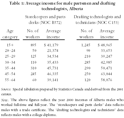
For example, Table 1 reports incomes by age (for Alberta males) for two occupations that are commonly recommended as retraining possibilities: partsman (NOC-S B572) and drafting technologist/technician (NOC-S C153). It can be seen there that annual incomes rise continuously from the youngest age group, 20-25, to the second oldest group, 45-54, before declining slightly.

Table 1

If it has been recommended that, say, a 40 year-old male retrain to enter one of these occupations, the economic expert is faced with determining which of the income levels from Table 1 best represents the income at which the plaintiff will begin his new career. If experience in the occupation, or movement along a career ladder, are important determinants of income, then we would expect that the newly-trained worker would begin at one of the lower incomes suggested by the census data.

Perhaps with his greater maturity the 40 year-old would not start at the income level of a 20-25 year-old; but with no experience in this occupation, it seems unlikely that he would start at the income of a 40 year-old. Fortunately, statistical evidence has recently become available that can help us to determine the impact of a change in career.

Most importantly, Arthur Goldsmith and Jonathan Veum[*] have used a detailed survey that followed 1400 young workers from 1979 to 1996 to compare the effects of additional years of experience on wages when individuals: remained in the same occupation and industry, remained in the same occupation but moved between industries, remained in the same industry but changed occupations, and changed both occupations and industries.

What they found was that the value that was placed on previous experience was approximately the same for all individuals except those that had changed both occupation and industry. In their words:

…experience acquired while a real estate agent is
valued similarly as tenure at other occupations, such as
accounting, within the real estate industry. In addition, the
experience as a real estate agent is valued similarly to
tenure at other industries, such as the pharmaceutical
industry, if continuing in the occupation of sales. If the
real estate agent becomes an accountant in the pharmaceutical
industry, however, the experience as a real estate agent is
of less value than that within accounting or the
pharmaceutical industry. (p. 442)

Referring to the examples in Table 1, Goldsmith and Veum’s findings suggest that the 40 year-old who retrains as a partsman may be able to earn an income comparable to that of a 40 year-old partsman with 15 years experience, if the retrained individual remains within his previous industry. For example, if an individual who had previously worked on oil rigs becomes a partsman in a shop that provides equipment to oil rigs, he can be expected to obtain a starting salary much higher than he would have obtained if he had become a partsman in an automobile dealership.

We would suggest that Goldsmith and Veum’s findings be interpreted in the following way: First, if the plaintiff’s injuries require that he/she retrain for both a new occupation and a new industry, the starting salary should (normally) be selected from the 25-29 year-old census category. This allows for the finding that previous experience is of limited importance, while avoiding the confounding effect that the incomes of 20-24 year-olds will be biased downwards by issues of immaturity.

Second, if the plaintiff’s injuries require that he/she retrain for a new occupation in the same industry he/she worked in prior to the accident, it should be assumed that the experience gained in the previous occupation will be, in large part, transferable to the new occupation. This does not necessarily mean that a 40 year-old plaintiff should be assumed to start his/her new career at the income level of an experienced 40 year-old in that occupation. Most importantly, plaintiffs often experience residual mental and physical difficulties that will reduce their earning capacity below that of the individuals represented in the census data. Also, however, it must be recognised that Goldsmith and Veum’s results referred to individuals who had changed occupations voluntarily; that is, to individuals who had chosen new occupations that met both their interests and their aptitudes. Plaintiffs often are not provided with that opportunity. As the new occupations for which they are retraining are not those that they had chosen when they were healthy, it is possible that they will not perform as well as individuals who had chosen those occupations voluntarily.

Finally, it must be recognised that Goldsmith and Veum’s findings are only suggestive. They can only be interpreted to indicate that, on average, when uninjured individuals make mid-career changes within a given occupation or industry, they tend not to suffer appreciable losses of earnings. They provide less information about specific individuals, particularly those who make significant career changes because of injury. We strongly suggest, therefore, that counsel request an opinion from a vocational psychologist concerning the impact that the injuries suffered by the particular plaintiff in question will have on that individual’s earning capacity. Specifically, if the psychologist recommends that the plaintiff retrain for a different occupation or industry, does the psychologist believe that that individual will be able to begin the new career at a salary that is comparable to other individuals of his/her age? Or will the plaintiff be forced to enter the new career at a salary lower than that of otherwise comparable individuals?

Footnotes

* Goldsmith, A.H. and J.R. Veum (2002). Wages and the Composition of Experience. Southern Economic Journal, 69(2), 429-443. [back to text of article]

leaf

Christopher Bruce is the President of Economica and a Professor of Economics at the University of Calgary. He is also the author of Assessment of Personal Injury Damages (Butterworths, 2004).

Derek Aldridge is a consultant with Economica and has a Master of Arts degree (in economics) from the University of Victoria.

The Discount Rate Revisited

by Christopher Bruce, Derek Aldridge, Kelly Rathje, and Hugh Finnigan

This article first appeared in the summer 2005 issue of the Expert Witness.

In the Autumn 2000 issue of this newsletter, we conducted an extensive review of the various methods of measuring the real rate of interest, or discount rate, and presented evidence concerning the movement of those measures over the period 1995-2000. (That article is available on our website, at economica.ca/ew53p1.htm.)

That survey was subsequently updated in our Winter 2001/02 and Spring 2003 issues. What we found in both of those updates was that interest rates had begun to fall relative to the historically high levels that had persisted over most of the 1990s.

At the time of our Spring 2003 article, we concluded that the best estimate of the long-run discount rate was 3¼ percent. But we also argued that, as interest rates on short-term bonds and GICs were lower than those on longer term investments, it would be appropriate to employ an interest rate of 2¼ percent on the first five years of any investment.

The primary purpose of this article is to examine nine additional quarters (27 months) of data to determine whether the trend we observed in our earlier articles has continued, or whether a revision in our recommended interest rate is appropriate. We also report on recent changes to Ontario’s mandated discount rate; and we revisit the question of whether forecasts of future interest rates should be based on information about past interest rates or on information about current, long-run interest rates.

Revised Data

Instead of providing tables of data comparable to those presented in our earlier articles, we now present a chart that shows the trend in interest rates since 1995. The complete data set can be found on our web site (see www.economica.ca/ew102p1.htm). Figure 1 shows the trend in real interest rates on government bonds of various term lengths, as well as the rate of return on real rate of return bonds.
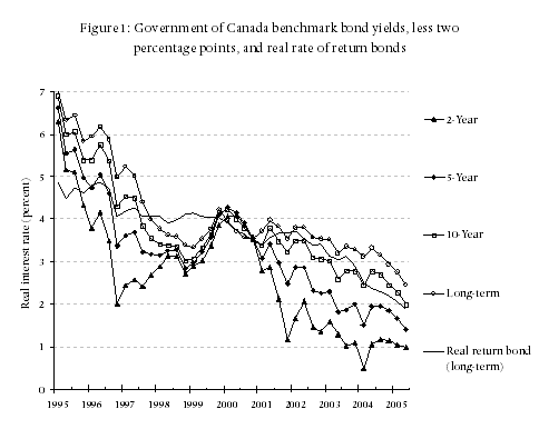
Figure 1

Note: We deduct two percentage points from the “nominal” or observed interest rates to reflect inflation anticipated by investors. As the Bank of Canada has managed to keep the core rate of inflation within a small band around this target since the early 1990s, and as it has been the stated intention of not only the Bank of Canada but most other central banks (most notably that of the European Union) to keep the inflation rate at that level, there is now virtual unanimity among investors that two percent will be the long run rate of inflation in Canada. Accordingly, it can be concluded that investors have been acting as if the real rate of interest is the observed, nominal rate less two percent.

The data in Figure 1 indicate that real rates of interest have continued the downward trend that began in 1996/97. Whereas we concluded two years ago that long-term real interest rates were approximately 3¼ percent and short-term rates approximately 2¼ percent; it now appears that real rates have fallen substantially below those levels. In particular, note that the rate of return on 10-year Government of Canada bonds, net of the 2 percent expected rate of inflation, is now below 2 percent and has not exceeded 3¼ percent (our earlier prediction of the “long-term” rate) since early 2002. Even the real rate on long-term (30-year) Government of Canada bonds has fallen below 2½ percent in the most recent quarter. And the rate of return on real rate of return bonds is now below 2 percent and has not been above 3 percent since mid-2003.

Although we do not show the comparable interest rates on guaranteed investment certificates (GICs), we have examined them and they are consistently lower that the rates of return on bonds. For example, the real rates on 1-year GICs have been consistently negative since late-2001, meaning that investments in one-year GICs are not keeping pace with inflation. The real rate on 5-year GICs has been below one percent for all but two of the last eight quarters and has not exceeded two percent since early 2002.

Forecasting the Real Rate of Interest

For some time now, Economica has been arguing that current interest rates, net of the two percent expected rate of inflation, provide the most reliable basis on which to predict future interest rates. Some other economic experts in Western Canada disagree with us, and base their forecasts on information about historical interest rates. We consider their position to be unjustified. We explain why here:

The continued dramatic fall in interest rates.

First, as a glance at Figure 1 will indicate, the real rate of interest in the last decade has fallen continuously and dramatically: the long-term rate has fallen from about 7 percent to below 2½, while the short-term rate has fallen from about 6 percent to below 1 percent. Clearly, any prediction that was based on an average of the figures in this period (or any other period extending back to the early 1980s) would seriously overstate the rates that will be available to a plaintiff investing his or her award today.

It is important to note that although rates are low by historic standards, today’s investors who seek the security of investments comparable to government bonds and GICs cannot avoid these low rates. The fact that average interest rates over the last 30 years were much higher does not help today’s plaintiff-investor. Even if one believed that long-term real rates will rebound to (say) 3.5 percent in the next 5-10 years, the best that today’s investor will be able to do is place his funds in 5-10 year investments earning 1.5-2 percent and then hopefully reinvest at the higher 3.5 percent rate. This of course will not yield nearly the same result as if he had been able to invest at 3.5 percent right from the start.

Economic theory.

Second, the fall in real interest rates is consistent with macroeconomic theory. Specifically, many macroeconomists are arguing that the relatively high real interest rates that were observed in the 1980s resulted from the high volatility in expectations concerning the nominal rate of inflation. That is, when inflation is unpredictable, investors who place their funds in long-term bonds face a considerable amount of uncertainty. If inflation proves to be higher than expected, the real rate of return that they realise may be very low or even negative. To compensate for this uncertainty, investors demand a relatively high expected rate of return. Conversely, when inflation becomes predictable, as has happened in the last five to ten years, investors face much less uncertainty and are willing to accept lower real rates of return. Accordingly, there is sound reason to believe that, as long as the Bank of Canada maintains its current course[*] (which it is expected to do), both nominal inflation and real interest rates will remain at the low levels that have been observed recently.

Furthermore, most economists believe that real interest rates will be higher in a period in which governments run large deficits – and, therefore, have to borrow heavily – than in those in which revenues exceed expenditures. As is well known, although the Canadian government ran sizeable deficits in the late 1980s and 1990s, it has now adopted a goal of achieving a balanced (or, even, surplus) budget. Again, this leads us to believe that real interest rates will be lower in the future than they were in the 1980s and 1990s.

The actions of large, institutional investors.

Most of the bonds reported in Figure 1 are purchased by large, institutional investors, such as pension funds. That these investors are willing to purchase, say, ten-year bonds paying a real rate of approximately two percent, or real rate of return bonds that are paying below two percent (as of the second quarter of 2005) indicates that they do not anticipate that they can obtain better rates of return on other secure investments. That is, regardless of whether private investors actually purchase the government bonds identified in Figure 1, the returns on those bonds indicate that the institutions that base millions of dollars of investment on their predictions of the financial markets are forecasting that real rates of return will remain low in the foreseeable future. (If expert institutional investors anticipated that rates on secure investments will average, say 3½ percent over the next ten years, then they would not buy bonds that pay only two percent, and the Government of Canada would be forced to adjust its bond rates.)

A future increase in rates will have little effect on most plaintiffs.

Even if real interest rates were to increase substantially in the next ten years or so, (against expectations), that would have relatively little effect on the investments of many plaintiffs, for two reasons. First, it is the rates of return that are available today that will dictate the average rate that plaintiffs will be able to obtain over at least the first 5-10 years of the period of their loss. As noted above, if rates increase in the future, the best that today’s plaintiff can do is place his funds in 5-10 year investments at today’s low rates and then later reinvest at the (hopefully) higher future rates. Even if rates return to their historical average, this investment approach will still yield an average rate of return that is below the historical average. Second, since most plaintiffs will need to begin consuming their award immediately (to replace their lost income and fund their costs of care), the most substantial portion of the interest that they will earn on the investment of their awards will occur in the first half of their period of loss, before they have drawn down much of their capital (that is, during the period in which they are funding most of their annual losses from interest income). If the period of loss is 20 years or less (like most plaintiffs), then the interest they earn in the first ten years will have a much greater impact on their investments than the interest they earn in the next ten years. Thus a return to higher interest rates after 10 years or so will have only a small impact on these plaintiffs. For plaintiffs with a period of loss that is only ten years or less, future increases in interest rates will have almost no effect on their investments.

Note that one implication of relying heavily on current interest rates is that it requires that we change our discount rate assumption more frequently than if we simply relied on historical averages. However, making changes to our discount rate assumption does not imply a weakness in our methodology. To do otherwise would result in us using interest rates that we know are inconsistent with the rates that are actually available to plaintiffs. Even if one believed that over the long-term, real interest rates will average (say) 3 or 3½ percent, it does not necessarily follow that our discount rate assumptions should remain fixed. This is because (as we explained above), the rates of return over the next ten or so years will have a substantial impact on the investment results of most plaintiffs. Thus, it is important to account for the rates that are available to plaintiffs now, as well as the rates that will be available (on average) over the long-term.

Ontario’s mandated discount rate

Following a detailed review, Ontario (in year 2000) revised its regulations concerning its mandated discount rate. The new methodology that was chosen yields a discount rate of 1.5 percent for the first fifteen years of any award and 2.5 percent for all years beyond that point. Specifically, Ontario’s revised regulation 53.09 states:

53.09 (1) The discount rate to be used in determining the amount of an award in respect of future pecuniary damages, to the extent that it reflects the difference between estimated investment and price inflation rates, is,

(a) for the 15-year period that follows the start of the trial, the average of the value for the last Wednesday in each month of the real rate of interest on long-term Government of Canada real return bonds (Series V121808, formerly Series B113911), as published in the Bank of Canada Weekly Financial Statistics for the 12 months ending on August 31 in the year before the year in which the trial begins, less 1 per cent and rounded to the nearest ¼ per cent; and

(b) for any later period covered by the award, 2.5 per cent per year. O. Reg. 488/99, s. 2; O. Reg. 263/03, s. 4 (1).

The average month-end rate of return on real rate of interest bonds from September 2003 through August 2004 was 2.58 percent. Deducting one percentage point and rounding to the nearest quarter percent yields a mandated discount rate of 1.5 percent for trials that occur in 2005. Given the rates on real rate of interest bonds since September 2005, we can also be almost certain that Ontario’s mandated discount rate (for the first 15 years of loss) will fall to 1.0 percent for trials that occur in 2006.

As discussed in an earlier article (see “Ontario’s Mandated Discount Rate – Rule 53.09(1)” that appeared in the Autumn 2000 issue of the Expert Witness), we have a concern with Ontario’s policy of deducting one percentage point from the one-year average of the rate on real rate of return bonds. What is perhaps more interesting is their finding that 2.5 percent reflects the long-term real rate of interest. This rate is lower than the long-term rate we have been using, though it is consistent with the current rate on long-term Government of Canada bonds.

Conclusion

Our review of the empirical and theoretical sources suggests that it would be appropriate to adjust our discount rate assumption. We also propose to make a change in how we apply our discount rate assumptions in our calculations. Whereas we previously assumed that the real rate of return on all of a plaintiff’s investments would be 2.25 percent for the first five years and 3.25 percent thereafter, we now assume that for income required in the first few years, an investment will be made at short-term rates, while for income needed in the more distant future, investments will be made that will earn the predicted long-term rates. Below we will further explain the approach we will use for our calculations, and then we will outline the discount rate assumptions we will use.

To illustrate the effect of this approach, note that a child plaintiff who will not experience a loss of income for ten years will manage to earn a relatively high rate of return because he will be able to invest in “long-term” investments, and he will be more likely to benefit from possible future increases in interest rates. On the other hand, an older plaintiff who will experience a loss of income over the next five years only, will not be able to benefit from long-term investments or from possible increases in interest rates. She will face the low rates available on short-term investments.

Consider the following example of a plaintiff who will incur a loss of income of $10,000 seven years from now. If she is compensated for the future loss today, she could use her award to purchase a government bond with a seven-year term, and not touch the award until it is needed in seven years, when the bond matures. We will see in Table 1 (below) that such a bond has been paying about 2.2 percent, net of inflation over the last two years. This plaintiff will not need to invest at the lower rates offered by shorter-term assets, but she will also not benefit from the rates offered on longer-term bonds, nor will she benefit from a possible future increase in interest rates. To invest her award in secure assets she faces two options: she can make successive short-term investments in hopes that the rates will increase in the near future, or she can make a longer-term (seven-year) investment and accept the interest rate that is available to her. Given her investment-obligations as a plaintiff, we would expect that that latter option would be more appropriate. Even if she chose the former option we would not expect her overall return to improve, unless we knew that rates would increase in the near future. (And if it was known that rates will increase in the near future, then this increase would already be reflected in the current rate of return offered on seven-year bonds.)

For our calculations we will choose an average rate of return that will be earned on investments that are held until each future year of the period of loss. For example, we assume that the portion of the plaintiff’s award that is held for seven years to compensate her for her loss in year 7 will earn an average rate of return of 2.2 percent. Similarly, we assume that the portion of the plaintiff’s award that is held for 15 years to compensate her for her loss in year 15 will earn an average rate of return of 3.0 percent. And so forth.

To obtain the discount rates for use in our calculations, we propose to take an average of the most recent two years of quarterly interest rates (using two years of monthly rates would yield the same results), for the Government of Canada benchmark bond yields for 2-, 3-, 5-, 7-, 10-year, and long-term bonds. After deducting two percentage points for anticipated inflation and rounding to the nearest tenth of a percent, this will give us our assumed real interest rates for various future terms. We assume the one-year rate is the same as the reported two-year rate, and for the “in-between” years we simply extrapolate. We assume that the long-term rate applies to year 15 and beyond. The rates that result from this approach are shown in Table 1.
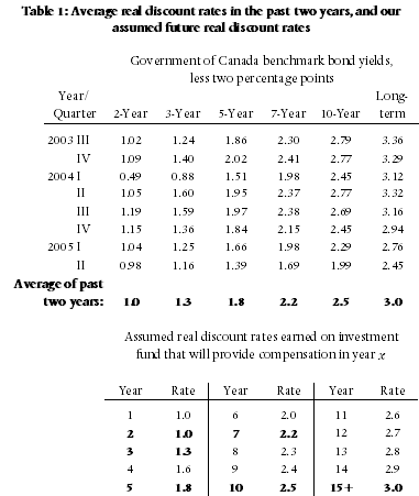
Table 1

Note that we believe that the rates proposed in Table 1 (above) remain conservative (that is, they may understate future losses) since they reflect interest rates that have been available over the past two years, instead of only the rates that are available now (even though only the rates available now can be assured to today’s investor).

Footnotes

* Since approximately December 1993, the Bank of Canada has successfully maintained a policy of keeping inflation at a two percent target (the midpoint of its 1-3 percent target range). [back to text of article]

leaf

Christopher Bruce is the President of Economica and a Professor of Economics at the University of Calgary. He is also the author of Assessment of Personal Injury Damages (Butterworths, 2004).

Derek Aldridge is a consultant with Economica and has a Master of Arts degree (in economics) from the University of Victoria.

Kelly Rathje is a consultant with Economica and has a Master of Arts degree (in economics) from the University of Calgary.

From 2003 through 2005, Hugh Finnigan was a consulting economist at Economica, with a Master of Arts degree from the University of Calgary.
Spring 2005 issue of the Expert Witness newsletter (volume 10, issue 1)

Contents:

  • The Impact of Disability on Earnings: Reliable Data
    • by Christopher Bruce
    • From his analysis in his previous article, Dr. Bruce concluded that, to be reliable, evidence must be based on data sets that meet two criteria: First, the number of observations must be large enough that one can be certain that a representative sample has been drawn. And, second, the data set must include individuals drawn from all of the comparison groups that are of interest.

      In this article Dr. Bruce uses these two criteria to identify a set of research reports that he considers to be reliable; and he summarises the findings of these reports with respect to the impact that each of spinal cord injuries, chronic pain, visual and hearing disabilities, and brain damage have on both education and earnings.

The Impact of Disability on Earnings: Reliable Data

by Christopher Bruce

This article first appeared in the spring 2005 issue of the Expert Witness, though it is based on a paper that Dr. Bruce presented at the Canadian Bar Association national conference, “Hot Topics in Litigation,” in Toronto on April 16, 2005.

In a previous article in this newsletter, “The Reliability of Statistical Evidence Concerning the Impact of Disability,” I argued that the courts should be very cautious when relying on evidence concerning the effects of disability on earnings. In this paper, I summarise some of the statistics on this factor that I consider to be reliable.

Criteria

Before a data set can be used with confidence, it must meet two criteria. First, the number of observations must be large enough that one can be certain that a representative sample has been drawn of all relevant populations. This means, first, that the sample must include individuals both with and without the disability in question; and, second, that the sample of the disabled population must be large enough that the results are not affected by accidental inclusion of unrepresentative individuals. For example, if one Canadian in a thousand has a particular disability, it might be necessary to survey one Canadian in three hundred in order to obtain a sample of sufficient size (in this case, one hundred) to ensure that a few “outliers” did not affect the statistical findings. Second, the observations must be drawn in a sufficiently random manner that the researcher can be confident that the individuals in the sample are representative of the population of interest. For example, it might not be appropriate to rely on a follow up survey of one hundred patients from a hospital that attracted an unrepresentative group of patients – unless the plaintiff was known to fall into that group.

My experience suggests that there are two sources of data that best meet these criteria: data sets constructed by national statistical agencies, such as Statistics Canada and the U.S. Bureau of Labor Statistics, and certain of the large, longitudinal studies – such as the National Longitudinal Survey or the Panel Study on Income Dynamics – that have been conducted by reputable research institutes in the United States. When employed by well-trained researchers, using appropriate statistical techniques, these data provide information on which the courts can rely. In the following sections, I summarise some of the studies that I believe meet the criteria set out above.

Spinal Cord Injuries

One of the most widely-studied groups of victims is those who have suffered from spinal cord injuries – paraplegia and quadriplegia. Fortunately, within the dozens of studies that have been conducted, there is a small set that employ large, reliably-drawn sets of data and appropriate statistical techniques. I particularly recommend three of these:

  • Bruce, Christopher (2004) Assessment of Personal Injury Damages, 4th Edition, (Butterworths: Toronto), Chapter 8 (with Hao Wang).
  • Krause, J. Stuart, et. al. (1999) “Employment After Spinal Cord Injury: An Analysis of Cases from the Model Spinal Cord Injury Systems” Archives of Physical Medicine and Rehabilitation 80, November, pp. 1492-1500.
  • Krueger, Alan, and Douglas Kruse (1995) Labor Market Effects of Spinal Cord Injuries in the Dawn of the Computer Age, (National Bureau of Economic Research: Cambridge, MA), Working Paper 5302.

The data in my book are the most representative of the total population (both disabled and non-disabled) as they are taken from the 1990 Canadian census. However, as the census identified individuals by impact of disability rather than cause, I was forced to use “unable to walk or carry light objects” as my disability category, rather than “spinal cord injured.” The Krause et. al. and Krueger and Kruse data were less representative than mine, as the U.S. census does not provide detailed information about disabled individuals. Instead, both studies relied on concerted efforts by research groups to gather data without government assistance. This meant that, although both were able to obtain large data sets that specifically concerned individuals with spinal cord injuries, they were unable to ensure that their data were truly randomly drawn.

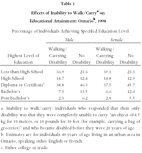
Nevertheless, the three studies provide compelling evidence concerning the impact of spinal cord injuries on labour market outcomes. First, because of the size and breadth of my sample, I was able to divide my data between those who had been injured before they were 20 years old and those who were injured later. This allowed me to investigate the effect that “inability to walk” had on the educational attainment of young disabled individuals. I found that non-disabled individuals were approximately twice as likely to complete a university education as were disabled; and were correspondingly much less likely to drop out of high school. (See Table 1.)

Table 1

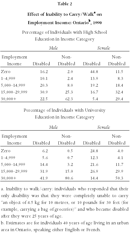
Conversely, by restricting a second sample to those who became disabled after they had completed their education, I was able to investigate the effect of “inability to walk/carry” on earnings, holding education constant. Here I found, first, that the disabled were much more likely than the non-disabled to be earning either no income or subsistence wages. Among those with high school education, for example, 26.3 percent of disabled males and 68.7 percent of disabled females earned less than $5,000 per year (in 1990), whereas the comparable figures for the non-disabled were only 4.4 percent and 20.1 percent, respectively. (See Table 2.)

Table 2

Second, there was a dramatic difference between the probabilities that the disabled and non-disabled would have earnings in the highest income category. Even after “correcting” for age, sex, educational level, province of residence and a number of other variables, I found that those who were unable to walk were less than half as likely to earn over $30,000 as were those who reported no disability.

Krause, et. al., lacking data concerning the non-disabled, could only comment on the factors that affected the probability that a spinal cord injured individual would be able to find employment. Most importantly, they found that if the individual had been employed at the time of the injury, he/she was almost four times as likely to be working after the injury as if he/she had not been so-employed; and that those spinal cord injured with a university education were three times as likely to be employed as were those with less than a high school education.

Krueger and Kruse were able to provide information concerning both employment and earnings. Perhaps their most important finding was that, even after allowing for age, sex, education, race, and marital status, victims of spinal cord injury were much less likely to be employed than were the non-disabled. Specifically, whereas approximately 75 percent of the non-disabled in their study were employed, the comparable probabilities for the sub-categories of spinal cord injury were: incomplete paraplegic, 42.2 percent, complete paraplegic, 29.5 percent, incomplete quadriplegic, 27.6 percent, and complete quadriplegic, 22.2 percent. That is, they found that the most common outcome of spinal cord injury was that the victim became competitively unemployable.

They were also able to confirm Krause’s finding that individuals with university education were three to four times more likely to be working after injury than were those with high school education or less. Whereas only 10 to 15 percent of those in the latter group were employed, 50 to 60 percent of those in the former were working post-injury.

With respect to those who did manage to obtain employment, Krueger and Kruse found that the earnings of the spinal cord injured were approximately 40 percent lower than the earnings of a matched set of non-disabled individuals. For each injured individual who had been working before his/her injury, Krueger and Kruse identified a comparable individual at the same workplace who had not been injured. They then compared the earnings of the injured and non-injured workers approximately five years after the injury occurred. Of this differential, approximately half arose because the injured parties worked fewer hours per week and half because they had lower hourly earnings.

Chronic Pain

In a recent paper, Crook et. al. ? Determinants of Occupational Disability Following a Low Back Injury: A Critical Review of the Literature,” Journal of Occupational Rehabilitation, 12 (4), December 2002, 277-295. surveyed the entire literature on the effects of chronic pain. Interestingly for the argument I made in my previous paper, they found that less than one percent of research studies they identified (19 out of 2,170) met a basic set of criteria for methodological reliability. Those studies reported that victims returned to work more quickly (following the onset of chronic pain) the younger they were, the greater was the availability of job modifications, the sooner they were referred for treatment, the less pain they had from standing and lying, and the greater was their flexibility. Males returned to work more quickly than females; and individuals with previous hospitalization or previous episodes of back pain took longer to return to work than did those without such histories.

Crook’s survey also found that females and older workers were the most likely groups not to return to work at all. Other factors making it more likely that patients would not return to work were: relatively large numbers of children at home and a lack of control over the workplace.

Finally, pain was more likely to be persistent, the older was the worker and the greater was the degree of depression.

Visually Impaired/Blind

I was able to identify only two studies of the visually impaired that provided data from large, statistically reliable sources.

  • Bruce, Christopher (2004) Assessment of Personal Injury Damages, 4th Edition, (Butterworths: Toronto), Chapter 8 (with Hao Wang).
  • Blackorby, Jose, and Mary Wagner, (1996), “Longitudinal Postschool Outcomes of Youth With Disabilities: Findings from the National Longitudinal Transition Study,” Exceptional Children 62 (5), 399-413.

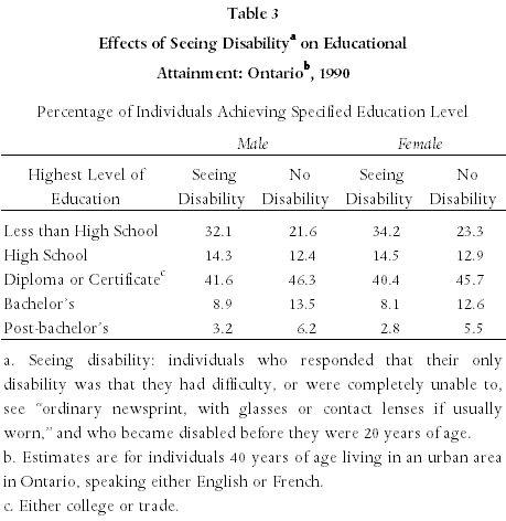
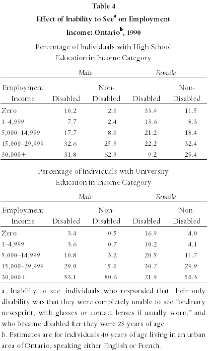
The first of these is my own study, using Canadian census data for individuals who reported that they had difficulty, or were completely unable, to see “ordinary newsprint, (with glasses or contact lenses if usually worn).” The Blackorby and Wagner study is based on a survey of over 8,000 students who had been enrolled in special education classes at high schools across the United States and who had been interviewed between three and five years after completing secondary school. Although this group included individuals with other disabilities, it also included a substantial portion who reported “visual impairment.”

The main findings from my research are reported in Tables 3 and 4. There it is seen that although those with a seeing disability are only slightly less likely to complete advanced education than are the non-disabled, the former are much more likely to be found in the lower portion of the income distribution than are the latter.

Table 3

Table 4

These findings were confirmed in large part by Blackorby and Wagner. They found, for example, that 57 percent of visually impaired students had attended some form of postsecondary school, only slightly less than the 68 percent of non-disabled students. Nevertheless, they found that only 29.4 percent of the visually impaired were competitively employed – less than half of the 69 percent figure for the non-disabled.

Hearing Impaired/Deaf

The two most reliable sources of information about the hearing impaired are the same as for the visually impaired:

  • Bruce, Christopher (2004) Assessment of Personal Injury Damages, 4th Edition, (Butterworths: Toronto), Chapter 8 (with Hao Wang).
  • Blackorby, Jose, and Mary Wagner, (1996), “Longitudinal Postschool Outcomes of Youth With Disabilities: Findings from the National Longitudinal Transition Study,” Exceptional Children 62 (5), 399-413.

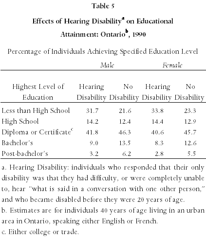
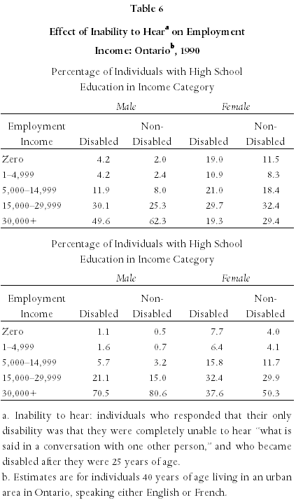
The main findings from my research are reported in Tables 5 and 6. As with the visually impaired, it is seen that those with a hearing disability are only slightly less likely to complete advanced education than are the non-disabled. The impact of hearing disabilities on income are much less, however, than is the impact of visual disabilities.

Table 5

Table 6

Again, these findings were confirmed in large part by Blackorby and Wagner. They found, for example, that 60 percent of hearing impaired students had attended some form of postsecondary school, only slightly less than the 68 percent of non-disabled students (and slightly more than the 57 percent of visually impaired). Similarly, they found that only 43.5 percent of the hearing impaired were competitively employed – almost 50 percent more than among the visually impaired.

Brain Injury

Two studies of the effects of brain injury appear to be based on large, representative samples. They are:

  • Dikmen, S. et al. (1994). “Employment Following Traumatic Head Injuries,” Archives of Neurology, 51 (2), 177-186.
  • Roberts, A.H. (1970) Severe Accidental Head Injury: An Assessment of Long-Term Prognosis (London: Macmillan)

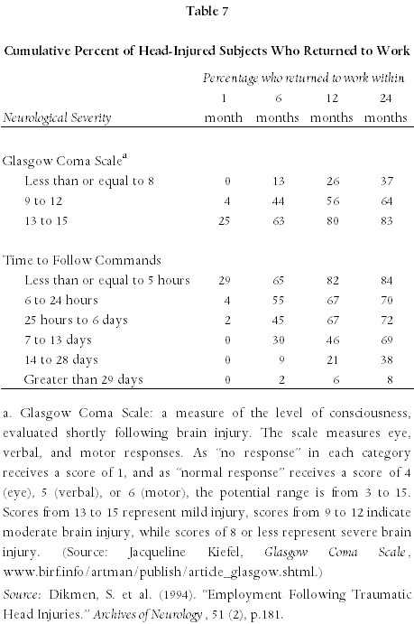
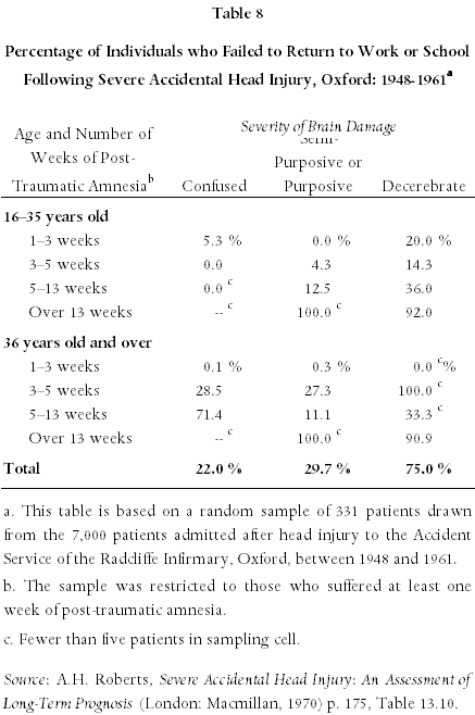
Both studies provide data concerning the probability of returning to work, given various measures of brain damage that are commonly available from medical reports. (See Tables 7 and 8.) As would be expected, the more severe is the injury, the lower is the probability that the individual will return to work. Also, the Roberts study found that workers were less likely to return to work, the older they were.

Table 7

Table 8

Discussion

In my experience, most medical/psychological evidence concerning the impact of disabilities on education, employment, and earnings takes two forms. First, the expert offers an opinion concerning the possibility that the plaintiff will be able to return to competitive employment. Second, the expert may offer an opinion concerning the (set of) occupation(s) for which the plaintiff can re-train if he/she cannot return to his/her pre-injury occupation. Typically, in the former case, no mention is made of the probability that the plaintiff will enter competitive employment, and in the latter case, no mention is made of the possibility that the plaintiff will work fewer hours than before the accident. Furthermore, in neither case will the expert make reference to the studies that provide statistics concerning these probabilities. Yet, as I have argued here, if one is diligent, and cautious, it is possible to identify numerous studies that provide reliable information on many aspects of the disability-employment relationship.

leaf

This article is based on a paper that Dr. Bruce presented at the Canadian Bar Association national conference, “Hot Topics in Litigation,” in Toronto on April 16, 2005.

leaf

Christopher Bruce is the President of Economica and a Professor of Economics at the University of Calgary. He is also the author of Assessment of Personal Injury Damages (Butterworths, 2004).