Autumn 1998 issue of the Expert Witness newsletter (volume 3, issue 3)

Contents:

  • The Economics of Negligence Rules
    • by Christopher Bruce
    • As a continuation of his series, Christopher Bruce expands on the use of economic analysis in tort law. He argues the economic approach can also be used to cast light on the development of the tort rules of negligence.
  • Using Industry Growth Rates to Update Census Occupational Earnings Figures
    • by Kris Aksomitis
    • In this article Kris Aksomitis discusses the method used to adjust average income figures derived from the Census from past dollars to today’s dollars. He compares average incomes taken from the 1996 Census with adjusted figures from the 1991 Census to illustrate the accuracy of these adjustments.
  • Drawbacks to the Use of “Preliminary” Estimates
    • by Thomas R. Ireland
    • In this article, Dr. Thomas Ireland explains, in letter format, the dangers of relying on preliminary estimates. Dr. Ireland is a well-known economist and is involved in the assessment of personal injury damages.
  • Timing, Turning Bad into Good
    • by Heber G. Smith
    • In this article Heber Smith sheds light on how to survive the markets with global events such as the Asian Crisis and the Russian meltdown. This article is of particular interest to holders of structured settlements.
  • The MacCabe Judgment: Allowing the Use of Earnings Statistics for Males When Estimating the Future Income of a Female
    • by Derek Aldridge
    • In this article, Derek Aldridge explains how the MacCabe judgment is important from the economist’s view. What does the judgment imply about future cases involving injured or deceased females? There are many questions unanswered.

The MacCabe Judgment: Allowing the Use of Earnings Statistics for Males When Estimating the Future Income of a Female

by Derek Aldridge

This article was originally published in the autumn 1998 issue of the Expert Witness.

On October 5, the Alberta court released its decision in the case of MacCabe v. Westlock RCSSD #110 et al (action: 9303 05787). The judgment is important for many reasons, though the most important aspect from an economist’s point-of-view is that it recommended the use of male earnings statistics to estimate the future earnings potential of a female. In particular, it was found that Ms. MacCabe would have followed a career path similar to that of the average male. That is, the court concluded that she would not have taken significant amounts of time out of the workforce for child rearing, and she would not have worked part-time. Therefore, it found that earnings statistics for males should be used to predict what her income would have been.

Some of the most important sections from the decision (related to the male/female income statistics issue) are reproduced here:

[para468] Clearly the evidence establishes that the exceptional individual characteristics of the Plaintiff are such that her abilities would have commanded the equivalent salary of her male counterparts. She would have established a strong attachment to her career. The use of male wage tables is justified. In any event, I am of the view that any award which I grant to the Plaintiff should not and cannot be solely determined by her gender.

[para469] It is entirely inappropriate that any assessment I make continues to reflect historic wage inequities. I cannot agree more with Chief Justice McEachern . . . in Tucker, supra, that the
courts must ensure as much as possible that the appropriate weight be given to societal trends in the labour market in order that the future loss of income properly reflects future circumstances. Where we differ is that I will not sanction the “reality” of pay inequity. The societal trend is and must embrace pay equity given our fundamental right to equality which is entrenched in the constitution. . . .

[para470]  . . . The Court cannot
sanction future forecasting if it perpetuates the historic wage disparity between men and women. Accordingly, if there is a disparity between the male and female statistics in the employment category I have determined for the Plaintiff the male statistics shall be used, subject to the relevant contingencies. . . .

[para481]  I agree with Dr. Bruce that absent
the accident, the Plaintiff would have been committed to her career and there would not have been a significant withdrawal from the labour force. . . .

So what does this imply about future cases involving injured or deceased females? It seems clear to us that if it is accepted that a young female would have followed a career path similar to that of the average male (in which she works full-time and does not take significant amounts of time out of the workforce for child rearing), then it follows that income statistics for males should be used to estimate her pre-accident income. (We discussed this issue in the Autumn 1997 issue of the Expert Witness.)

But what if it is found that a young woman would have followed a traditional female career path? In this case we suggest that using income statistics for females will still probably underestimate the true income path, but using those statistics for males will probably overestimate the true income. The reality likely lies somewhere in between the two alternatives. However, the MacCabe judgment appears to leave open the possibility that earnings statistics for males could be used even for female plaintiffs who would have followed “traditional” female career paths. It may be the case that the courts will choose to apply earnings statistics for males, regardless of the evidence about the woman’s likely career path – as a sort of “social justice” choice (Recall paragraph 469 of MacCabe: “I will not sanction the ‘reality’ of pay inequity.”)

However, the same argument could possibly apply to other situations in which a certain group of people earn less, on average, than the average male. For example, it is well-known that, on average, Natives earn less than non-Natives. From the MacCabe decision it may follow that one should use average income statistics for males to estimate the potential income of a young Native male (or female), with no adjustment to account for the reality that the average Native earns less than average non-Native. Conversely, perhaps the defense could argue that a person who has been disfigured in an accident should not be compensated for the “appearance-discrimination” component of his loss of income because that would be an endorsement of the “reality” of discrimination. If the court chooses to correct for the reality of pay inequity, then this could raise some difficult issues for those of us involved in loss of income cases.

leaf

Derek Aldridge is a consultant with Economica and has a Master of Arts degree (in economics) from the University of Victoria.

Timing, Turning Bad into Good

by Heber G. Smith

This article was originally published in the autumn 1998 issue of the Expert Witness.

In the past, my financial advisors were quick to remind me how splendidly they were handling my finances. More recently, however, they are somewhat sheepish discussing the more than modest shrinkage in my meager retirement assets, referring to such world events such as the Asian Crisis and the Russian meltdown as possible causes.

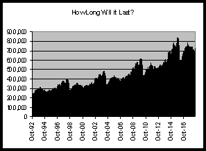
Upon closer scrutiny, I discovered what may have been long apparent to investors more skilled than I — that portfolio performance isn’t always a function of management but of timing. During a bull market, most equity positions increase in value but during bear markets, the converse is usually true. To make matters worse, an investor who is dependent on a market-based portfolio for needed income, will find that the concept of dollar cost averaging works against him/her when withdrawing regular fixed dollar sums from equity portfolios during a bear market. The timing of such sells to satisfy fixed income requirements dictates that, on average, more assets are sold low than are sold high. In order, therefore, to enable a personal injury client to reap the income required for the settlement duration, we suggest that an action settled during the early stages of a bull market is best. Consider the following chart (below left), which illustrates regular withdrawals of $1,200 per month adjusted for a 25% tax rate when $250,000 is invested in the TSE 300 in the fall of 1992. The result is an increasing portfolio value.

Figure 1

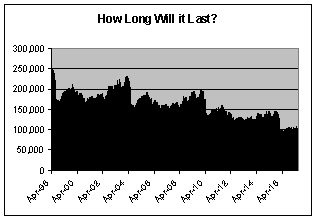
Figure 2

* An assumption of stock market cyclicity of 6 years was used so that the same TSE 300 data repeated every 6 years leaving the starting time as the differentiating variable.

Conversely, a different picture appears if the same $1,200 per month adjusted for tax is withdrawn from the same sized portfolio beginning in the spring of 1998 (above right). Under this scenario, the personal injury claimant has the added anxiety of wondering whether his funds may dissipate before their specified time. Unfortunately for the claimant, a personal injury settlement date is not dependent and timed for receipt according to stock market investment cycles.

Hope in the ability to time markets need not be as critical a factor. By using a combination of a structured settlement and dollar cost average purchases in the TSE 300, one can reduce risk and, during volatile markets, virtually assure an increase in settlement withdrawal periods.

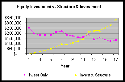
Consider providing for a claimant’s income requirements via a structured settlement for the first 16 years and the purchase of a second annuity to support the dollar cost average purchases in the TSE 300 over the same period. The following graph depicts the value of the investment fund at the end of the 16 years when purchased in the spring of 1998 in comparison to the value of the investment fund purchased by using an annuity and dollar cost averaging over the same period.

Figure 3

So what makes it all work? It is the combination of financial planning tools; diversification and risk reduction that go a long way to turn what could be bad timing into good (or at least better timing). But the biggest factor is the imputed contribution made to the settlement by Revenue Canada Taxation in the way of tax forgiveness on the interest element of the annuity contract supporting the settlement. In combination, the above enables a claimant to grow the investment fund prior to withdrawals thereby increasing the number of payment periods and reducing anxiety due to dissipating funds.

leaf

Heber Smith is the principal of Smith Structured Settlements Inc. a structured settlement and annuity brokerage with offices in Calgary and Vancouver. He is also a partner in Structured Settlement Software, a firm that provides tax driven software to the American structured settlement industry.

Drawbacks to the Use of “Preliminary” Estimates

by Thomas R. Ireland

This article was originally published in the autumn 1998 issue of the Expert Witness.

In a recent posting to an e-mail service for economists who act as expert witnesses, Thomas Ireland, a well-known American economist, wrote about an issue that usually receives little attention — the dangers of relying on preliminary estimates. Although we do not agree with all of Dr. Ireland’s conclusions, we feel that many of the points he raises are of sufficient interest to be reported here. Accordingly, we reprint the following letter, with Dr. Ireland’s permission.

Fairly recently, I sent a letter to an attorney who had requested that I avoid producing any report except the final report of my opinions. This involved a situation in which I was asked to prepare preliminary estimates, but might not be asked to finalize my reports until several months later. It occurred to me that the text of this letter might be of interest to fellow practitioners.

Dear Attorney:

The purpose of this letter is to explain why I feel that I need to develop preliminary reports. I write my reports in the form of a letter addressed to an employing attorney unless asked to use a different format. In a very real sense, however, I write them to myself as well. This is for three reasons. First, in developing most reports, I must make a number of very small decisions that do not have a large impact on my damage assessments, but are things I need to remember at depositions and at trials. In my tables, is “age” shown as the plaintiff’s age at the start of the year, or on his birthday during the year? What issue of USFinancial Data was the source of my discount rate? How did I annualize the earnings figure in the year of injury? And so forth. If I am preparing a preliminary table, I need this kind of information if I pick up the file three months later and am trying to figure out exactly what I did to produce the exact numbers in my tables.

Second, my reports are not full of fluff that is designed to make it look like I did more work than I did (like many other economist reports that I see). They are simple narratives explaining what I was asked to do, what assumptions I was asked to make, what materials I was given to prepare, what I took from those materials, what additional assumptions I made, what my opinions are and how my tables work to produce those opinions. In effect, as I am writing the narrative parts of my report, I am subjecting my calculations to a step by step logical consideration of whether I have performed those steps correctly. I find mistakes much more easily when writing my narrative than by staring at tables or spreadsheets.

In other words, I need to develop a preliminary report to remember what I did and to check my calculations at the time I create them. Attorneys hate to see what they regard as unnecessary documents that might come back to haunt them. But the cost of not creating documents may be serious and much more embarrassing errors or failures of memory. For me to prepare extensive notes rather than narratives would take more of my time and be more likely to result in errors. Further, the notes themselves then become a document that could cause more trouble than a narrative. As I write my narratives, even in a preliminary report, every word is considered from the standpoint of whether I would want to be cross examined about the meaning of that word. I try to be very precise in my narratives, but am much less careful in notes I write to myself. I now typically type all of my handwritten notes as a part of deposition preparation to make sure that I have no handwritten notes that I do not understand.

Third, I want attorneys to read my narratives to see whether I may have misinterpreted any of the information they have provided to me. Sometimes important facts are given to me by telephone and I may have written them down incorrectly. Sometimes documents that I have been given create misleading impressions. I have found that attorneys are very good at picking up errors that relate to demographic facts in my reports. That is a very important part of the process of checking the validity of my analysis.

Perhaps a fourth reason is that right after I write a report, I see what I intended to write, but not necessarily what I did write. Several weeks later, I will see what I did write and be able to catch things that I could not have caught at the time I wrote a report.

The bottom line here is that if you ask me not to produce preliminary reports, you are asking me to take a greater chance of making an important mistake or being unable to explain how I arrived at one of the values in one of my tables.

leaf

Dr. Thomas Ireland is a professor of economics at the University of Missouri at St. Louis.

Using Industry Growth Rates to Update Census Occupational Earnings Figures

by Kris Aksomitis

This article was originally published in the autumn 1998 issue of the Expert Witness.

The most reliable source of information about the incomes of specific occupations is the census. Unfortunately, census data are collected only once every five years — and income data are not published until three years after they are collected. (For example, income data from the 1995 census were not available until July of 1998.)

As a result, if census data are to be used, some method must be found for updating those data between the most recent census year and the year in which the information is required. For example, to use census income data in early 1998 (before the release of the 1995 census data), estimates of 1998 earnings had to be based on data from the 1990 census. This updating is achieved by increasing the relevant census figure by an estimate of the percentage increase in earnings between the most recent census year and the year in question.

The data series which is most often used to obtain this estimate is Statistics Canada’s Annual Estimates of Employment, Earnings and Hours (Cat. 72F0002XDE). This series reports estimates of average weekly earnings by
industry. Hence, as the desired figure is income by
occupation there is some concern that growth rates based on the Statistics Canada occupational earnings series will fail to provide an accurate estimate of the desired increase.

To my knowledge, no one has attempted to test whether industry growth rates provide an accurate estimate of occupational growth rates. That is the purpose of this article.

Here, I calculate the growth rates of incomes in various
occupations between the 1990 and 1995 censuses and compare those growth rates to estimates of those rates, which have been obtained from the annual growth rates of
industry earnings.

Methodology

The purpose of the article is to test the accuracy of using industry growth rates to predict average earnings for specific occupations. As such, the procedure uses the following steps:

  • First, a number of occupations were selected as a basis of comparison. The selection process was fairly arbitrary, but an attempt was made to include occupations from a number of distinct industries.
  • Second, data were collected for the chosen
    occupations from the 1990 Census and the 1995 Census. These figures represent the actual annual average incomes for these occupations in the respective years. The ratio of the incomes in 1995 and 1990 were calculated for each occupation.
  • Third, data were collected on industry income growth rates. These figures were calculated from average weekly earnings for the specific industries in question, and were used as proxies for salary growth rates within those industries.
    [Note that the calculated figures for both industry and occupation are simple percentages and not compound growth rates. For example, the calculated “all occupations” growth factor of 13% means that earnings increased 13% in total over the 5 years, or slightly less than 2.5% compounded annually. For each industry or occupation, the growth factor was calculated by dividing the value of 1995 earnings by the value of 1990 earnings.]
  • Fourth, the “actual” rate of growth of earnings for each occupation was compared to the growth rate of earnings from the industry that I believed to be most closely related to the occupation in question. In the table, below, I refer to these industry growth rates as “estimated” rates of growth as they represent our best estimates of the growth of occupational earnings.
  • Finally, the actual occupational growth rates were compared with both the estimated growth rates and the average, “all-industry” growth rate.

Analysis

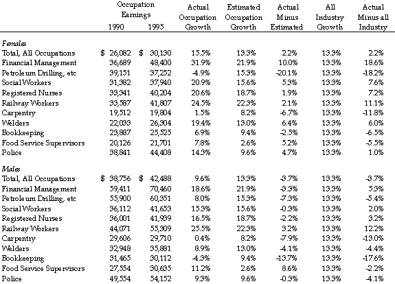
The table presents the results. A number of interesting observations can be drawn from the data. The first, and most important observation, is that the industry specific growth rates provide a better estimate than the overall average growth rate in all but five cases.

From this observation, it can be argued that, for the most part, the industry-specific estimated growth rates provide a better estimate of earnings growth than do the average growth rates for the entire economy. Of the occupations I examined, only for male food service supervisors did the average growth rate provide a significantly better estimate than did industry-specific growth.

A second observation is that the estimates provided by the industry specific growth factor is quite accurate in the majority of the cases. For example, in 12 of the 22 cases, the estimated earnings are within 5.1% of the actual earnings. This indicates that, in these cases, the annual compound growth rate predicted by the estimate is within 1% of the actual annual growth rate in earnings.

Some of the errors can be explained by the small sample size of the occupations. This would appear to be the case, for example, with respect to female petroleum drillers. In other cases, for example male bookkeepers, it may be that individuals were spread among so many industries that no estimate from a single industry could be expected to prove accurate.
[Interestingly male bookkeepers and female drillers were the only two occupations of those I’ve examined whose
earnings were lower in 1995 than in 1990. In every other case, actual earnings increased over the 5-year Census period and the earnings estimates by the model provided a reasonable estimate of actual earnings.]

A final observation from the data is that the correlation between actual and predicted earnings seems highest in occupations which are characterised by a high degree of unionization. For example, accurate estimates were obtained for police, social workers, registered nurses and railway workers.

Conclusions

Overall, it seems that industry-specific growth rates provide a reasonable estimation of occupational growth. In the majority of cases, the specific industry growth rate provided a better estimation of actual earnings growth than did the general economy growth rate. Further, in many cases the industry wage growth rate provided an excellent proxy for the specific occupational growth rate, especially in those occupations that were most highly unionized and clearly defined as part of that industry.

Figure 1

leaf

Kris Aksomitis was a research associate with Economica Ltd. and an MA student in Economics at the University of Calgary.

The Economics of Negligence Rules

by Christopher Bruce

This article was originally published in the autumn 1998 issue of the Expert Witness.

In the summer 1998 issue of this newsletter, I introduced the academic discipline of “the economic analysis of tort law.” I argued in that issue that the traditional legal analysis of torts employs an ex post orientation. That is, legal scholars traditionally assume that the function of tort law is to compensate victims for harms that have already occurred. Economists, on the other hand, argue that the evolution of torts can better be understood if one uses an ex ante paradigm. In this paradigm, the courts behave as if they are less concerned with the resolution of the cases before them than they are with the establishment of precedents that will affect future behavior. In particular, economic analysis “predicts” that the courts will prefer those rules that encourage parties to select cost-minimising behaviors.

In the summer 1998 article, I provided examples of a number of situations in which the courts appeared to have made explicit use of ex ante reasoning. In this article, I will argue that the economic approach can also be used to cast light on the development of the tort rules of negligence.

Legal Versus Economic Analysis

If one adopts the proposition that the function of tort law is to compensate accident victims, it is difficult to rationalise the rules of negligence. Those rules require that the victim show that the defendant was negligent before compensation will be ordered. But as many defendants are not negligent, many victims are not compensated. Why would a body of law whose purpose was to compensate victims contain a major “escape clause” which would deny compensation to a large percentage of victims?

One could begin to answer this question by modifying the traditional argument. Perhaps tort law is not designed to compensate all accident victims, just those who are deemed “worthy.” But this begs the questions of who is worthy and why it is that the “worth” of the victim should be defined by the behavior of the defendant.

I will argue in this article, that negligence rules can better be understood if we view their purpose as being cost-minimisation. Under this approach, a party will only be found to have been negligent (and therefore potentially liable to pay damages) if he or she had failed to take some precaution for which the cost was less than the benefit (measured in terms of accident costs avoided). That is, I will argue that the function of the tort rules of negligence is to send signals to potential (future) “injurers” that if they fail to take appropriate precautions, they will be made to bear the costs that result.

Negligence Rules: an Economic Exposition

The economic model can best be understood using a numerical example. Assume the following “facts,” (based, loosely, on Anderson v. County of Ponoka [1980] 12 ALR 320):

  • One of the stop signs at the intersection of two country roads is knocked over sometime on Saturday evening.
  • The County responsible for those roads becomes aware of this on Sunday morning but decides to wait until Monday morning to replace the sign, in order to save $100 overtime pay to its road crew.
  • Sunday evening, Mr. A, unaware that the sign is missing, assumes that he has the right-of-way, enters the intersection without slowing, and collides with Ms. B’s car.
  • The two cars and their occupants suffer damages which total $25,000.
  • At trial, the court accepts the evidence of a traffic expert that the probability, per day, that such an accident will occur is 3/1,000 if there is no stop sign in place and 1/1,000 if there is a stop sign.

Was the county negligent? Economic analysis predicts that the court will say “no.” Why? Assume that rural stop signs are frequently knocked down on Saturday evenings. If the relevant highway departments wait until Monday to replace the stop signs, there will be three accidents every 1,000 times a sign is knocked down. Hence, there will be $75,000 damages for every 1,000 such occurrences. ($75,000 = 3 x $25,000.) If the counties replace the stop signs immediately, the number of accidents will fall to one in every 1,000 occurrences, reducing the accident costs to $25,000, a saving of $50,000. But, in order to obtain that “saving,” counties will have to send out 1,000 repair crews at an overtime cost of $100 each, or $100,000 in total. The $50,000 “saving” will have cost $100,000.

Put another way, the average cost of precautions, per event, will be $100 and the average benefit of those precautions (measured in terms of accident costs saved) will be (2/1,000) x $25,000, or $50. As the economic model predicts that the court will only encourage behaviour whose cost is less than the benefit, the economic prediction is that the court will not find the county to be negligent in this case.

It can be seen from this case that three factors are predicted to enter the court’s calculations:

  • the cost to the defendant of taking a precaution to avoid the accident, (C);
  • the probability that a precaution which could have been taken by the defendant would have prevented the accident, (P); and
  • the expected cost of the accident, (A).

In particular, it is predicted that the defendant will be found to have been negligent if there was some precaution, not taken by the defendant, whose cost was less than the cost of the accident multiplied by the decrease in the probability of an accident which would have occurred had that precaution been taken. In algebraic terms, the party is found negligent if C < (A x P).

Is the Law Consistent With the Economic Model?

In the U.S., this prediction was confirmed in one of the leading cases on negligence, U.S. v. Carroll Towing. In that case, Justice Learned Hand concluded that negligence was to be found only if the burden (cost) of precautions was less than the probability of the accident multiplied by the gravity (cost) of the accident — precisely the formulation which I derived above from the economic model.

In British/Canadian jurisprudence, confirmation of the prediction is less direct, but persuasive nevertheless — sufficiently persuasive that in recent editions of Canadian Tort Law Allen Linden has organised his discussion of the rules of negligence around the “Learned Hand rule.” In Wagon Mound No. 2, for example, the court concluded that a party could be found negligent even if the probability of an accident was low as long as the cost of the accident was high. Arguably, it was the court’s view that the cost of the accident multiplied by the probability that it could be avoided should be weighed against the cost of avoidance in order to determine negligence — again, precisely the prediction made by economic reasoning. Other leading cases which are consistent with the economic model include Bolton v. Stone, Priestman v. Colangelo, and Reibl v. Hughes.

Applying Economic Analysis to the Law

Many “day-to-day” cases also employ reasoning which is consistent with the economic approach to the determination of negligence. For example, in Hewson v. City of Red Deer (1977) 146 DLR (3d) 32 (Alta. CA), a City employee left the keys in the ignition of a bulldozer. Subsequently, the bulldozer was stolen and driven into the side of Hewson’s house. The City was found not to be negligent largely because (a) the bulldozer was left two blocks from Hewson’s house; (b) it was left at midnight; and (c) the operator was absent for only 25 minutes. All three of these factors suggest that the probability of an accident was quite low. And the first factor suggests that the average damages which might occur if the bulldozer was stolen were low (because the bulldozer would have to be driven a long distance before causing any harm.)

In Weaver v. Buckle (1982) 35 AR 97 (Alta. QB), Weaver (a child) ran out in front of Buckle’s car and was injured. The court implied that it would not normally have found Buckle to be negligent for causing this accident. However, as the road was narrow, it found that he should have been driving more slowly, to take account of the general conditions of that road. The court concluded that if he had been driving more slowly, the probability that this accident would have occurred would have been reduced substantially. Buckle was found 60 percent liable. In economic terms, this finding suggests that it is not simply this accident which determines the “costs of an accident” (A, in my terminology). Rather, it is all accidents which might have been prevented had the defendant taken additional precautions.

In Jordan v. Schofield (1996) 148 NSR (2d) 104 (NSSC), Schofield’s 7 year-old son played with a lighter and caused a fire in an apartment building belonging to Jordan. The court concluded that Schofield was not negligent. Although parents are responsible for taking “reasonable” precautions to watch their children and to put harmful things out of their way, at some point the costs of additional precautions become prohibitive. Parents will not be found negligent for failing to take precautions beyond that point. For example, parents will not be negligent for leaving children unattended around “ordinary” dangers (such as knives or scissors) for a few minutes. They may, however, be negligent for leaving their children unattended around such dangers for longer periods of time, or for leaving them for only a few minutes around more dangerous items (such as fires burning in fireplaces). In economic terms, the cost of taking additional precautions is to be weighed against the probability that an accident will occur if those precautions are not taken.

To conclude, given that no Canadian court has formally adopted the “Learned Hand rule” it would be difficult to base an argument before our courts on economic reasoning alone. Nevertheless, if one accepts that the three components of the “Learned Hand Rule” (C, P, and A) play an implicit role in the determination of negligence, an understanding of their function may help to clarify the legal analysis in difficult cases.

leaf

Christopher Bruce is the President of Economica and a Professor of Economics at the University of Calgary. He is also the author of Assessment of Personal Injury Damages (Butterworths, 2004).