The Impact of Poor Health on Retirement Age

by Christopher Bruce

This article first appeared in the autumn 2007 issue of the Expert Witness.

In personal injury cases, plaintiffs often argue that their disabilities will induce them to retire early and, therefore, cause a reduction in lifetime earnings. As such claims are largely based on the plaintiff’s own testimony, it is often difficult for the courts to determine whether the claim is credible and, if so, to identify the number of years by which retirement will be accelerated.

The purpose of this article is to assist the court in these determinations by providing a survey of the academic literature on the effects that health limitations have on the age of retirement. As the first edition of my textbook, Assessment of Personal Injury Damages (Butterworths, 1985) contains a survey of the early literature on this topic, I concentrate in this paper on articles published since 1990.

This yields a set of eight studies. Of these, two (Disney, for Britain, and Campolieti, for Canada) reported only that a negative change in health or disability status among individuals over 50 had a “significant” negative effect on the age at which those individuals retired.

Of the remaining studies, two provided data concerning the impact of alternative levels of health status on the probability that 50-65 year-olds would be working. Au, Crossley, and Schellhorn, using Canadian data from 2000-2001, reported that even a minor change in health status, from “very good” to “good,” would reduce the probability of employment by 10 percent. (See Table 1.) And a change from “excellent” to “poor/fair” could reduce employment by as much as 40 percent (among males).
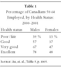
Table 1

Similarly, Cai and Kalb, using Australian data from 2001, found that a change in health status from “excellent” to “poor” would reduce the probability that individuals would be in the labour force by approximately 16-18 percent. (See Table 2.)
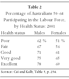
Table 2

At age 55, these reductions in probabilities imply that individuals in poor health will retire between one and two years earlier than those in very good health. This is consistent with Gustman and Steinmeier’s finding, for the United States, that individuals who were “limited in the kind or amount of work” in which they could engage could be expected to retire two years earlier than those not so-limited.

Berger and Pelkowski, for the United States, and Jimenez-Martin, Labeaga, and Prieto, for Spain, also found impacts that were similar to those found by Campolieti and Au, et. al., but using somewhat different measures of health status.

Jimenez-Martin et. al. reported that 55-65 year-old individuals with “severe disability” were 14.6 percent less likely to be employed than were the non-disabled, and that those with “very severe disability” were 28.5 percent less likely to be employed than were the non-disabled.

Berger and Pelkowski found that among 51-61 year-old couples in which both the husband and wife had (at the beginning of the study period) been healthy and employed, the effect of a health problem was to reduce the probability that the wife would be working by 19 percent and that the husband would be working by 35 percent.

Finally, McGarry found that a change in health status from “good” to “fair” would reduce the probability that a 62 year-old would be working from approximately 45 percent to 40 percent.

To summarise, regardless of the country that is investigated, the evidence is clear: a reduction in health, from “good” to “fair or poor” will have a significant, negative impact on the probability that 50-65 year-old individuals will be working. Although the precise effect of such a reduction varies from study to study, there appears to be fairly consistent evidence that the average effect is to reduce the age of retirement by approximately two years (for example, from age 61 to age 59).

References

Au, D. W., T. Crossley, and M. Schellhorn (2005) “The effect of long-term health on the work activity of older Canadians.” 14 Health Economics, 999-1018.

Berger, M., and J. Pelkowski (2004) “Health and family labor force transitions.” 43 Quarterly Journal of Business and Economics, 113-138.

Cai, L., and G. Kalb (2006) “Health status and labour force participation: Evidence from Australia.” 15 Health Economics, 241-261.

Campolieti, M. (2002) “Disability and the labor force participation of older men in Canada.” 9 Labor Economics, 405-432.

Disney, R., C. Emmerson, and M. Wakefield (2006) “Ill health and retirement in Britain: A panel data-based analysis.” 25 Journal of Health Economics, 621-649.

Gustman, A., and T. Steinmeier (2000) “Retirement in dual-career families: A structural model.” 18 Journal of Labor Economics, 503-545.

Jimenez-Martin, S., J. Labeaga, and C. Prieto (2006) “A sequential model of older workers’ labor force transitions after a health shock.” 15 Health Economics, 1033-1054.

McGarry, K. (2004) “Health and retirement: Do changes in health affect retirement expectations?” 39 Journal of Human Resources, 624-648.

leaf

Christopher Bruce is the President of Economica and a Professor of Economics at the University of Calgary. He is also the author of Assessment of Personal Injury Damages (Butterworths, 2004).

Death and Retirement: Allowing for Uncertainty

by Christopher Bruce

This article first appeared in the autumn 2005 issue of the Expert Witness.

Assume that a plaintiff has begun to recuperate following a serious accident. If her injuries stabilize at their current level, she will suffer a loss of earnings of $20,000 per year. If, however, she has a relapse, her losses will increase to $40,000 per year. Her doctors tell you that there is a 50 percent chance that there will be a relapse (and a 50 percent chance that there will be no relapse).

How should the annual value of her loss be calculated? If damages are set equal to $20,000 per year, there is a 50 percent chance that she will be under compensated; whereas if she is paid $40,000, there is a 50 percent chance that she will be over compensated. (And if she is paid some amount between $20,000 and $40,000, there is a 100 percent chance that she will be incorrectly compensated.)

This conundrum, in which there is uncertainty about the outcome of future events, is common in the assessment of personal injury (and fatal accident) damages. Not only is there uncertainty about the future course of the plaintiff’s injuries, as in the example above, we also face uncertainty concerning the age at which the plaintiff will retire, the plaintiff’s life expectancy, the probability that the plaintiff would have (and will be) unemployed, and a host of other factors.

The general approach that virtually all financial experts take in such cases is to calculate the average outcome that would arise from the uncertain event, if the event could be repeated a large number of times. For example, if the injury described above was to be repeated 100 times (for example, if there were 100 plaintiffs with that same injury), we would expect that the plaintiff’s injuries would remain stable in approximately 50 cases, leading to a loss of $20,000 per case. In the other 50 cases, the plaintiff would suffer a relapse and her loss would rise to $40,000. Thus, the total annual loss, across all 100 cases, would be ((50 × $20,000) + (50 × $40,000) =) $3,000,000. The average annual loss would be $30,000; which could also be calculated by multiplying 50% times $20,000 and adding 50 % times $40,000. That is, the average value of a loss can be calculated by multiplying each of the possible losses by its probability and then adding the resulting numbers together.

But, as was noted above, $30,000 is guaranteed to be the “wrong” amount in 100 percent of cases. How, then, can it be justified? One simple answer is this: if the event in question is truly uncertain, the plaintiff should be able to use the $30,000 to purchase insurance that will compensate her fully regardless of which value turns out to be her true loss – either $20,000 or $40,000. The reason for this is that if the insurer issues, say, 100 such policies, it can expect to pay out $20,000 in 50 cases and $40,000 in the other 50, for an average of $30,000. (It will have collected $3,000,000 [= 100 × $30,000] and will have paid out $3,000,000 [= 50 × $20,000 + 50 × $40,000].)

Risk of Mortality

This type of calculation is most commonly used when dealing with the uncertainties associated with mortality. Take the extreme case in which there is a ? probability that a plaintiff will live exactly one year (and then die), a ? probability that he will live exactly two years, and a ? probability that he will live exactly three years. If he would have earned $60,000 per year but has now been left unable to work, his loss can be calculated using the technique described above. That is, there is a ? chance that he has lost one year’s income ($60,000), a ? chance he has lost two years’ income ($120,000), and a ? chance he has lost three years’ income ($180,000); for an average of $120,000 (=? × $60,000 + ? × $120,000 + ? × $180,000).

Alternatively, in such cases, it is sometimes possible to use a “rule of thumb” to estimate the loss. Given the probabilities in the preceding example, it can be shown that, on average, the plaintiff will live two more years before dying. (2 = ? × 1 + ? × 2 + ? × 3) That is, his life expectancy is two years. His expected loss can then be calculated as the sum of his losses over that life expectancy, or $120,000 (= 2 × $60,000). Note, however, that this approximation works best if the losses are approximately the same in each year, as it was here. (If the annual loss is significantly different in the first year than, say, the third year, this approach yields a biased estimate.)

What is clear is that it would be inappropriate to mix together the two calculation techniques. It is not appropriate, for example, to estimate the loss by multiplying each of the first two years’ losses by their associated probabilities and assuming that the loss continues for only two years. That would produce an “estimated” loss of only $60,000 (=? × $60,000 + ? × $120,000), $60,000 less than the true loss.

Retirement Age

The techniques described here can also be used to estimate the effect of uncertainties about the plaintiff’s retirement age. Assume, for example, that there was a ? probability that a 63 year-old plaintiff would have worked for exactly one year (i.e. to his 64th birthday) and then retired, a ? probability he would have worked two years, to his 65th birthday, and a ? probability he would have worked three years, to his 66th birthday. If he would have earned $60,000 per year while working, his loss, again, can be found from the formula: ? × $60,000 + ? × $120,000 + ? × $180,000 = $120,000; or by multiplying the average number of years to retirement by his annual earnings, to produce $120,000 = 2 × $60,000.

As with the mortality example, it would clearly be incorrect to multiply each year’s earnings by the probability it would occur and assume the individual would have retired at the average age, of 65. That would produce an “estimate” of, (? × $60,000 + ? × $120,000 =) $60,000, again, only half of the correct estimate.

leaf

Christopher Bruce is the President of Economica and a Professor of Economics at the University of Calgary. He is also the author of Assessment of Personal Injury Damages (Butterworths, 2004).

Complementarity in the Retirement Behaviour of Older Married Couples: An Update

by Daryck Riddell & Christopher Bruce

This article first appeared in the spring 2002 issue of the Expert Witness.

When forecasting the earnings streams of individuals over 50, one of the most important factors is predicted age of retirement. For example, changing the projected retirement age from 63 to 60, when the individual is currently 57, will decrease the future loss of earnings by approximately 50 percent.

It is often argued that one indicator of likely retirement age among individuals in this age group is the retirement decision of the plaintiff’s spouse. If a 57 year-old woman’s husband has already retired, that could indicate that she will retire earlier than would otherwise have been predicted.

Economists have observed three factors that might suggest a correlation between the retirement ages of spouses. These we refer to as: similarity of profiles, sharing of household finances, and complementarity of leisure.

Similarity of Profiles

Sociologists, psychologists, and economists have long observed that individuals choose mates who have socio-economic profiles similar to their own. If professionals marry professionals or high school leavers marry high school leavers, then the retirement ages of spouses will be similar, not because the retirement decision of one spouse affected the retirement decision of the other, but because the spouses’ decisions were affected by similar work-related influences.

Spouses who both worked in physically demanding jobs might both retire earlier than the population average, for example. Or spouses who were both self-employed – say, doctors or lawyers – might both retire later than average. In such cases, one might be tempted to conclude that because one retired soon after the other that the retirement of the first had “caused” the retirement of the second when, in fact, what had happened is that they had both been affected by the same external factors.

Sharing of Income

It has long been recognised in the economics literature that the likelihood that one spouse will leave the labour market will increase as the income of the other spouse increases. That is, the spouses of high income earners are more likely to be retired at any age than are the spouses of low income earners.

This observation suggests two hypotheses. The first of these is that if one spouse’s social security benefits increase, the “other” spouse will be more likely to retire. Evidence for this hypothesis has recently been obtained in two studies. Both Coile (1999) and Baker (2002) found that both wives and husbands were more likely to retire when the wives were eligible for income supplements than when the wives were not. It appears that wives’ retirement ages, however, were not strongly influenced by husbands’ availability of income supplements.

The second implication of “sharing of income” is that spouses’ retirement ages will be negatively correlated. That is, if one spouse has retired, the other will be less likely to retire. The reason for this is that when one spouse retires, that spouse’s income decreases (often, dramatically), thereby decreasing the probability that the other spouse will leave the labour force.

Complementarity of Leisure

A third hypothesis is that spouses will obtain greater pleasure from retirement if they retire together. In economic terminology, the benefits that one spouse obtains from leisure are complementary to the amount of leisure enjoyed by the other. For example, if the wife plans to spend her retirement travelling, she may expect to obtain more pleasure from her retirement if she anticipates that her husband will also be retired and will travel with her.

Clearly, this hypothesis suggests that spouses’ retirement ages will be positively correlated. That is, if one spouse retires, the other will be more likely to retire, as the second spouse will expect to obtain greater benefits from retirement leisure than if the first spouse had not retired.

Blau (1998) has recently provided evidence that this complementarity is an important factor in determining spouses’ retirement ages. His study examines the joint labour force behaviour of older married couples in the United States.

Using the Retirement History Survey (RHS), a longitudinal study that followed men and women who were age 58-63 in 1969, Blau constructs labour force histories for each married couple from the time the husband turned 55. The joint labour force status of the couple in any given time period is characterized by four possible states: both employed, neither employed, husband employed but wife not, wife employed but husband not.

The data set has some interesting features. Foremost among them is that the labour force transitions of one spouse are strongly associated with the labour force status of the other spouse. The wife’s exit rate from the labour force is 63 percent higher when the husband is not employed than when he is employed. Similarly, the husband’s exit rate when his wife is not working is 53 percent higher than when she is employed. Conversely, quarterly entry rates for both husband and wife are larger if the other spouse is employed rather than not employed.

Another feature is that the incidence of joint retirement is quite large. Between 11.4 percent and 15.7 percent of all couples exit the labour force in the same quarter and between 30.3 percent and 40.6 percent exit in the same year.

The key conclusion from this paper is that there is strong evidence of the preference to share leisure. This sample from the 1960s and 1970s shows a high incidence of joint retirement and a positive effect of non-employment of one spouse on the other spouse’s labour force exit rate, as well as a negative influence of non-employment of one spouse on the other’s entry (or re-entry) rate.

Summary

Economists have put forward three hypotheses concerning the likelihood that the retirement ages of spouses will be correlated. The first of these – similarity of profiles – suggests that, on average, spouses will retire at similar times because spouses tend to have similar socio-economic profiles. That is, the factors that act on retirement age independently of marital status will affect husbands and wives in similar manners.

The second hypothesis is that individuals will be more likely to retire, the higher is their spouse’s income. This hypothesis suggests that there will be a negative correlation between spouses’ retirement ages. When one spouse retires, family income will decrease and the second spouse will be provided with an incentive to remain in the labour force.

Finally, if the leisure activities of husband and wife are complementary, there will be a positive correlation between spouses’ retirement ages. Recent evidence suggests that this effect has been a significant determinant of retirement ages in the United States.

leaf

Daryck Riddell was a graduate student in Economics at the University of Calgary

Christopher Bruce is the President of Economica and a Professor of Economics at the University of Calgary. He is also the author of Assessment of Personal Injury Damages (Butterworths, 2004).

Spousal Influence on the Decision to Retire

by Scott Beesley

This article was originally published in the spring 1997 issue of the Expert Witness.

The decision to retire is influenced by several factors including income level, the available pension, company policy, legislation, employment opportunities, the need to help care for family members, health and the status of the spouse. Some interesting Canadian survey data and analysis regarding this last factor can be found in a book entitled The Road to Retirement, by Grant Schellenberg for the Canadian Council on Social Development (1994). A detailed statistical treatment of the issue, using U.S. data, is provided in the working paper Retirement in a Family Context: A Structural Model for Husbands and Wives by Alan Gustman and Thomas Steinmeier (National Bureau of Economic Research: Working Paper #94-4). We provide here a brief summary of the results reported in these studies and their implications for the calculation of lost future income.

Schellenberg listed four particular items which together constituted the spouse’s influence in the decision to retire. They were: the timing of the spouse’s retirement; the spouse’s health; the spouse’s income; and finally, pressure from the spouse to retire. His survey noted, for each item, the percentage of retired men and women who said that issue had been important in their decision to retire. The most notable finding was that for all four items, men were far less influenced by their spouse’s situation than were women. Less than 5 percent of retired men, for example, said that the timing of their spouse’s retirement had influenced their own timing, yet 22 percent of retired women had considered their husband’s situation in making their choice. The three remaining spousal issues were important to about 10 percent of women and an even smaller 2 to 6 percent of men.

An interesting change appeared when the same questions were put to men and women who, unlike the group discussed above, had not yet retired. This sample put a much higher weight on spousal considerations than those who had already left the workforce. Forty-five percent of women said that they expected their spouse’s time of retirement to affect their own, up from 22 percent, while the number for men rose from approximately 3 to 14 percent. The fraction of wives listing their husband’s health and income as important determinants rose even more, to about 40 percent. Similarly, the number of men who listed spousal health rose from 6 to 22 percent, while spousal income was expected to be important by 12 percent, which, while still small, is a significant change from the minuscule 2 percent reported by the retired group. The data quoted clearly reflect, in our view, the much increased importance of women’s income in total family income. One implication is that studies of the factors which determine retirement age will probably underestimate spousal influence, to the extent they are based on older data.

The American study by Gustman and Steinmeier (G & S) was a sophisticated attempt to quantify the effect of one spouses’ retirement decision on the other. In a somewhat striking contradiction of the results given for Canada by Schellenberg, G & S state that “There is some suggestion in the data that the wife’s retirement decision is not strongly influenced by the husband’s, but the husband’s decision is more strongly influenced by the wife’s.” One possible explanation is familiar to those who analyse survey data: Individuals do not necessarily do as they say they will, or (in hindsight) they report reasons for decisions which do not accurately reflect the real choices they made. Hence, while men (in the Canadian survey) might report that their wife’s decision to retire was or will be an insignificant factor in their own decision, the U.S. data, based on actual behavior rather than survey responses, suggests they are influenced, to a statistically meaningful degree, by their wives’ situation. It is perhaps not surprising that men would prefer to say their decision was independent of their wives’ status, if the alternative is to grant that they did not want to be alone at home while their wives continued to work. The authors of the U.S. paper suggest explicitly that perhaps men are unwilling to face housework alone, and they estimate that the effect of “wife being retired” is that husbands then behave as if they were two years older, and are hence more likely to retire themselves. The average change in time of retirement is found in a simulation to be only five months, however.

Another finding of G & S was that when the retirement decisions of couples are treated as jointly determined, a moderate tendency to retire together (or closer than would otherwise be expected) is evident. The alternative to joint determination would be assuming each spouse takes the other’s retirement age as given when determining their own, but this tends to lead to an overestimation of spousal influence.

Finally, we note that, though the tendency to retire at times which are closer together than the couple’s age difference was statistically significant in G & S, this factor is still much less important than the major issues listed at the beginning of this article, such as current income, available pensions, company and government policy and so on. It is these issues which we have historically considered when setting the retirement age in our calculations of lost income. No change in methodology is warranted as yet, though the Canadian survey suggests that spousal influence is increasing and may have to be accounted for in some future cases. If further research suggests that the “spousal effect” is (or will be) likely to produce differences of over a year on average, we can justify changing our assumptions at times. For example, if there is a strong financial incentive for the woman to retire at 58, and her husband would then be 60, we might plausibly assume he would retire immediately, rather than waiting until age 62, if his own income vs. pension calculation was not very age dependent. While this change would be minor for a 30 year old plaintiff (or survivor, in a fatal accident case), it could be quite important for someone in their 50s.

Of course, it would also be interesting (to an economist, at least!) to see if the above-mentioned difference between the opinions expressed in survey responses and the behavior found in real data is resolved.

leaf

Scott Beesley is a consultant with Economica and has a Master of Arts degree (in economics) from the University of British Columbia.