What is Econometrics?

Posted on December 1, 2000March 24, 2017 By economica

This article was originally published in the Winter 2000 issue of the Expert Witness.

Commonly, economic experts will testify that a particular characteristic of the plaintiff, such as his years of education or his marital status, is “correlated” with one of the factors that is of interest to the court, such as future income or retirement age. The branch of economics that seeks to determine whether such correlations exist is called econometrics. In this article, we explain briefly how econometric techniques work.

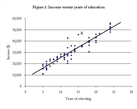
Assume that we are interested in determining whether the annual incomes that individuals earn are correlated with, or determined by, years of education. Assume also that 70 individuals have been observed and that for each individual, we know their number of years of education and annual income.

We have plotted the observations for these individuals in Figure 1. For example, individual A has 15 years of education and an annual income of $45,000.

When income levels are plotted against years of education, one would expect that the observations would be scattered, as seen in Figure 1. What the econometrician wishes to do is determine whether these scattered points form a “pattern.” One simple pattern that is often tested is that of a straight line. In this case, the formula for a straight line is:

I = a + b₁(E)

where I is income; a is a constant; b₁ measures the amount that education influences income; and E is years of education.

What the econometrician tries to do is to find the line which minimises the distances between the observations and the points on that line. The straight line which appears to meet this criterion with respect to the observations in Figure 1 has been drawn there. The formula for this line is

I = 6,850 + 2,000(E) (1)

This formula says that if the individual has 12 years of education, his income is predicted to be $30,850.

I = 6,850 + 2,000(12) = 30,850

It can be seen from Figure 1 that, in general, the observations lie fairly close to the line. For this reason, we would conclude that the hypothesis that education affects income is supported. Furthermore, because the “sign” on the 2,000 component of the equation is positive, we would also conclude that education has a positive effect on income. (In this case, each extra year of education appears to lead to 2,000 extra dollars of annual income.)

Equation (1), which investigates the effect which only one variable has on another, is not typical of the equations that are normally of interest to economists. Typically, for example, we would assume that there is a large number of factors, in addition to education, that will affect income. In that case, econometricians extend their equations to include numerous variables.

For example, suppose the economist has additional information about the age of each individual in the data set. This variable can also be added to the equation to help “explain” income. The equation would become:

I = a +b₁(E) + b₂(A),

where A is “age.” The resulting estimated equation might be something like:

I = 5,000 + 1,900(E) + 200(A) (2)

This model now indicates that for every extra year of education an individual has, they will earn an extra $1,900, on average, and for each additional year in age, there is an increase of $200. In other words, if an individual has a high school diploma, and is 34 years old, then the equation indicates on average, they will earn $34,600 (= 5,000 + [1,900 x 12] + [200 x 34]). Similarly, if an individual holds a bachelor’s degree (16 years of education), and is 34 years old, then the equation indicates that, on average, they will earn $42,200 (= 5,000 + [1,900 x 16] + [200 x 34]).

The variables used as examples to this point – income, education, and age – all share the characteristic that they can easily be measured numerically. Other variables which might influence the wage rate are less easily converted to numerical equivalents, however. Assume, for example, that our hypothesis was that incomes were higher in rural areas than in cities, or that men were paid higher incomes than women, all else being equal.

As econometric analysis is a statistical technique, it requires that the economist enter all of his or her information as numbers. The way that econometricians deal with this problem is to construct what are called “dummy variables.”

In this procedure, one of the observations is arbitrarily chosen to be the “reference variable” and it is given the value of 0 whenever it appears. The other observation is then given the value of 1. For example, if “female” was the reference category, then the dummy variable would be given the value 0 whenever the observed individual was female and would be given the value 1 whenever the individual was male.

Assume that this has been done and equation (2) has been re-estimated with a male/female dummy variable included. The new equation might look like:

I = 3,000 + 1,900(E) + 200(A) + 4,000(M) (3)

where M is 1 if the individual is male and 0 if she is female. The interpretation that is given to the value that appears in front of M in this equation is that income is $4,000 higher when the worker is a male than when the worker is female.

Alternatively, because the dummy variable takes on the value 0 when the worker is female, the relevant regression equation for females is simply equation (3) excluding the dummy variable:

I(female) = 3,000 + 1,900(E) + 200(A)

And because the dummy variable takes on the value 1 when the worker is male, the relevant equation for males becomes:

I(male) = 3,000 + 1,900(E) + 200(A) + 4,000(1)

= 7,000 + 1,900(E) + 200(A)

The income model is one example of how econometrics is used, and how it is useful to determine trends and relationships between variables. Other uses may include forecasting prices, inflation rates, or interest rates. Econometrics provides the methodology to economists to make quantitative predications using statistical data.

Kelly Rathje is a consultant with Economica and has a Master of Arts degree (in economics) from the University of Calgary.

Christopher Bruce is the President of Economica and a Professor of Economics at the University of Calgary. He is also the author of Assessment of Personal Injury Damages (Butterworths, 2004).

Evaluation of Harm to a Class of Individuals

Posted on December 1, 2000March 24, 2017 By economica

by Kelly Rathje

This article was originally published in the Winter 2000 issue of the Expert Witness.

When we are asked to estimate a claimant’s potential future income (without- or with-accident) we rely on two types of data – data specific to the individual, such as the claimant’s tax returns, and statistical data concerning individuals “similar” to the plaintiff, such as information drawn from the Census.

When the plaintiff is part of a common class of victims, however, it is possible to rely on more sophisticated statistical techniques to assess the impact of the injurious act. Such classes of plaintiffs might include, for example, victims of chemical or radiation poisoning in a factory or residential area or victims of sexual or physical abuse at a school.

In these cases, economists can rely on a technique known as econometric modelling (see the accompanying article from this newsletter) to determine whether the average income of the class of victims differs significantly from the average income of a similar group chosen at random from the population.

The difference may be determined by specifying characteristics, common to both groups, and examining how these factors influence income. Any difference in income not attributable to the specified characteristics could be attributed to the incident, and thus the loss of income due to the incident may be determined.

To use this method, an economist would need to gather data, do some comparative statistical analysis, and then apply the econometric model. These steps are outlined below.

Data

The data for the claimant’s group is most commonly compiled from information provided by the individuals within that group. The comparison group, which is to represent a random sample from the population, can often be obtained from broad data sources such as the census.

Using these sources, the economist would create two types of variables. The first of these are “numerical” variables; that is variables that can be measured using numerical scales. For example, if the economist is trying to identify the determinants of income, numerical variables might include age, years of education, and work experience.

The second set of variables, “dummy” variables, are variables that cannot be measured numerically. For example, these might include place of residence or sex of the individual. For example, if the economist wished to test the hypothesis that people in the Maritimes earned less than individuals in the rest of Canada (ROC), a variable might be created that divided the group between Maritimes and ROC.

Comparisons

Before any formal estimation is done, economists usually look at the raw data to see if any trends or relationships are present. Using the characteristics indicated above (age, place of residence, years of education, and current income), trends of interest to economists might be employment rates, average numbers of years of educational attainment, and average income levels for each group.

Econometric modelling

Using the characteristics outlined, an (econometric) equation is created to examine the factors that influence income. The equation, in its simplest form, might be as follows:

I = C + b₁[age] + b₂[maritimes] + b₃[claimants]

What this equation predicts is that income, I, will be determined by the individual’s age, place of residence, membership either in or out of the “claimant” group, and a fixed factor, C. In this equation, “age” is a numerical variable – it might take values such as 25 or 47 years old, for example.

“Maritimes” and “claimants” are dummy variables. In this case, “Maritimes” takes the value 1 if the individual lives in the Maritimes and 0 if he or she lives in the ROC; and “claimants” takes the value 1 if the individual is one of the plaintiffs and 0 if he or she was chosen from the random sample of other individuals in the population.

Once the data set has been collected, and the form of the equation has been identified, statistical techniques are applied to the data to estimate the “best” values of b₁, b_2, and b_3.

The data might suggest, for example, that the most likely relationship among the variables is:

I = 25,000 + 500[age]- 4,500[maritimes] – 20,000[claimants]

This indicates that for each year an individual ages, income increases by $500, on average; and that if the individual lives in the Maritimes, income will be, on average, $4,500 less than if that individual lives in the ROC. The above estimation also indicates that, on average, the claimant group will earn $20,000 less than average individuals in the population, all else being equal. For example, a 37-year-old, who lives in the Maritimes, and is not part of the claimant’s group would earn $39,000 (= 25,000 + 500[37] – 4,500[1] – 20,000[0]); and a 37-year-old, who lives in the Maritimes, and is a part of the claimant’s group would earn $19,000 (= 25,000 + 500[37] – 4,500[1] – 20,000[1]);

Now suppose the economist also has information on the employment status of each individual in both groups. The next step that may be undertaken is to estimate what an individual’s income would be given the above characteristics, but limiting the observations to employed individuals only. That is, the economist might control for employment status by including only observations at which the income is greater than zero. This would indicate how much of the difference in income, found in the first estimation, could be attributed to employment status. The resulting equation might be, for example:

I = 21,000 + 200[age] – 4,500[maritimes] – 12,000[claimants]

Given that I > 0

Recall from above, when considering both employed and unemployed individuals together, the equation indicated that the claimant’s group earned approximately $20,000 less than the random population. Now, controlling for employment, they are found to earn $12,000 less. This implies that $8,000 of the earnings gap between the plaintiff group and the general population can be explained by the higher unemployment rate of the former group.

Now suppose there is additional information regarding the education levels of the groups. The next logical step would be to add educational attainment as one of the explanatory variables. Thus, the equation would include the number of years of education, place of residence, age, and “claimant” status. This specification adds another explanatory factor to help predict income levels. Still controlling for employment status, the resulting equation might be:

I = 20,000 + 100[age]- 4,000[maritimes] + 2,000 [education] – 7,000[claimants]

Given that I > 0

This equation, given the known characteristics in this example, has the most explanatory power. It indicates to the economist that controlling for all the known variables, there still exists a difference in income of $7,000 between the claimants and an individual chosen at random from the general population, given that both individuals have the same characteristics.

Note, however, that this does not mean that the effect of the tortious act is, on average, $7,000 per year per claimant. First, remember that when no allowance was made for employment status or education, the average difference between the annual incomes of the claimants and members of the general population was $20,000. What the last equation predicts is that if we compare two individuals who have the same education and the same employment status, we will find that the “claimant” earns, on average, $7,000 less than the non-claimant. However, the effect of the tortious act may have been to increase the unemployment rates of the claimants and reduce their educational attainments (particularly if they were injured while they were minors). In that case, the $7,000 would represent the lower bound on the estimated impact of the injury.

Second, part of the income differential between claimants and non-claimants may be the result of factors that have not been taken into account in the equations. For example, assume that the claimants had all been harmed by the release of a toxic chemical. It might be that individuals who are susceptible to that chemical share some genetic factor that also reduces their abilities to earn income. If that genetic factor is not taken into account, the statistician may attribute the lower incomes of members of that group to the chemical when, in fact, that group would have earned lower incomes in any event.

Another drawback is that this method determines average incomes for the group, and thus, average differentials for the group. That is, the income differentials between the claimant group and the random group apply to the overall group, and not necessarily to each claimant. When the claimants are considered individually, the economist may find that some of the claimants are earning more than the average income predicted by the model; some are earning less income than the average income predicted by the model; and some are earning the same income the model predicted. However, on average, the group still has a reduction in earnings, when compared to individuals chosen at random from the population, with the otherwise same characteristics (other than the incident).

We were recently asked to determine whether there was economic evidence to support a claim that a group of individuals experienced a loss of income as a result of a common incident. We followed much of the same steps and methodology described here in determining: (i) whether an income differential existed; and (ii) the extent to which each of the known factors influence income. This methodology allowed a quantitative measure of the loss of income to be predicted, given the information provided by the group, and compared to a random sample of the population.

Kelly Rathje is a consultant with Economica and has a Master of Arts degree (in economics) from the University of Calgary.

Incorporating the Effect of Reduced Life Expectancy into Awards for Future Costs of Care

Posted on December 1, 2000March 24, 2017 By economica

by David Strauss, Robert Shavelle, Christopher Pflaum, & Christopher Bruce

This article was originally published in the Winter 2000 issue of the Expert Witness.

1. Introduction

Some of the largest personal injury and medical malpractice actions are brought on behalf of plaintiffs with chronic disabilities such as cerebral palsy, spinal cord injury, and traumatic brain injury. Such plaintiffs require extensive care and assistance for the rest of their lives, and the cost of future care is often the largest part of the claim.

There are three components to the calculation the present value of the cost of lifetime care:

A discount rate, specifying the interest rate at which it is assumed the lump sum award will be invested.
The dollar cost of providing care during each year. The rate at which this amount is assumed to grow over time is usually, though not necessarily, lower than the rate of discount.
A probability distribution specifying the probability that the plaintiff will live to each possible age in the future. In the calculation of the present value of future costs of care, the cost of care in each possible year in the future is multiplied by the probability that the individual will live to the age at which that cost is required. This is equivalent to reducing the required cost by the probability that the plaintiff will not live to a given age and, therefore, that the plaintiff will not require the assumed cost of care. [Note that this is analogous to multiplying the annual loss of income by the probability that the individual would have been working during that year, in order to capture the effect of the probability that the individual would have been unemployed.]

When the injury is not one that reduces life expectancy, the survival distribution that is used is that of the general population. The distribution can be obtained from an ordinary life table. (In Canada, this is the Life Tables 1990-1992.) Our interest here, however, is the case in which life expectancy is reduced, and it is no longer obvious how the annual survival probabilities should be chosen.

2. Alternative methods of calculating the impact of reduced life expectancy

Typically, medical opinion concerning reduced life expectancy is conveyed in the form of an average number of years of expected survival. For example, the medical experts might agree that the effect of the plaintiff’s injury is to reduce her life expectancy from 50 years to 30. The question we wish to consider here is how economists should incorporate this opinion in their calculation of the changes in annual probabilities of survival. A number of alternative techniques are commonly used.

Life certain – A very simple technique is to assume that the plaintiff will live exactly the number of years estimated by the medical experts and then die. For example, a 30 year-old who has a probability of 1.0 of living to each age between 30 and 50, and a probability of zero of living to any age beyond that, has a life expectancy of 20 years.

Although this technique is sometimes used to obtain to obtain very rough approximations, it is certain to produce estimates that exceed the true value by a substantial amount. The reason for this is that the life certain approach leaves all of the costs of care in the immediate future, (in this case, in next 20 years). In reality, the plaintiff has some probability of dying during the next 20 years and a corresponding probability of living more than 20 years. Hence, in reality, the costs of care should be reduced in the near future (to allow for the possibility that the plaintiff will die before needing them) and increased in the distant future (to allow for the possibility that the plaintiff will live beyond 20 years). But, as discounting reduces the present value of ‘distant’ costs more than it reduces the present value of ‘near’ costs, moving costs further into the future will reduce the discounted value of future costs.

Rating up – A simple method for obtaining a probability of survival to each possible age in the future is to find a “statistical person” who has the life expectancy of the injured plaintiff and to use that person’s probability distribution to represent that of the plaintiff. For example, consider a boy with severe cerebral palsy who has an agreed upon life expectancy of 20 additional years. The rating up method identifies the age in the general population at which the life expectancy is likewise 20 years.

According to the U.S. Decennial life tables, for example, this is 58 years. For each future age, the probability of survival for a 58 year old is substituted for that of the 5 year old. For example, the 5 year-old’s probability of living to age 15 is assumed to equal the probability that an average 58 year old would live to 68.

The attraction of this method is that it provides a probability distribution with the correct average, (here, 20 years). There is a problem, however: it is the wrong distribution. As the research literature makes clear, a child with a short life expectancy is subject to a fairly constant risk over the life span; he may well die in the next few years but he also has a reasonable chance of living another fifty. By contrast, the man of age 58 is at a relatively low risk over the next few years, but his risk increases steeply over the decades and he has almost no chance of surviving another 50 years.

Like the life certain method, the rating up method places too many of the costs of care in the immediate future, and too few in the distant future (relative to the “true” values). Hence, it systematically overestimates the present value of future costs of care.

Relative risk – In this approach, the economist multiplies all the age-specific mortality rates in a standard life table by a constant. The constant is chosen to result in the desired life expectancy, and is easily determined by trial and error. For example, if the annual probabilities that a male will die are multiplied by 47, the life expectancy of a 5 year-old will become 20 years. Although the argument is more complex than that made with respect to rating up, the relative risk approach also systematically overestimates the present value of future costs.

3. An Example

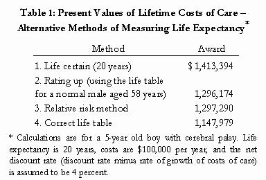
Table 1 shows lump sum awards for a 5 year-old boy with life expectancy 20 years who is to receive $100,000 for each remaining year of life. A discount rate of 4 percent is employed.

Table 1

The first row applies to a hypothetical child who will survive exactly 20 more years. This is the life certain distribution discussed above, and it leads to the largest award: $1,413,394. The second row is the result of rating up to age 58, which currently, perhaps, is the most widely used approach. The award of $1,296,174 is appreciably smaller than the $1,413,394 of row 2.

Row 3 uses the relative risk method. As indicated above, when the mortality rates of a standard life table are multiplied by 47, the life expectancy for a boy of age 5 years becomes 20 years. This is the multiplier that has been used. The resulting award of $1,297,290 is very similar to that obtained from rating up. Finally, row 4 gives the award when the correct life table, based on the latest evidence concerning cerebral palsy, is used. Use of the correct probability distribution leads to an award of $1,147,979.

In this example, both rating up and the relative risk method lead to awards that are too high by 13 percent, or approximately $150,000. And the life certain method leads to an award that is too high by almost 25 percent.

4. Comparison of the methods

The size of the discrepancy between the approximate methods and the correct survival distribution depends on several factors, of which the most important are the cost schedule, the discount rate, and the plaintiff’s life expectancy. Discrepancies will tend to increase as the rate of growth of costs decreases, as the discount rate increases, and as post-injury life expectancy falls.

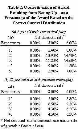
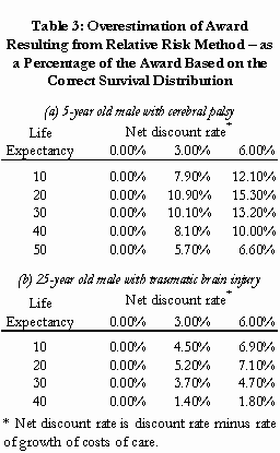
Tables 2 and 3 show the percentage overestimation for various discount rates with the rating up and relative risk methods, respectively. In addition to the case of a five year old with cerebral palsy (Tables 2a and 3a), we also consider that of a 25 year-old with traumatic brain injury and a life expectancy of 20 years (Tables 2b, 3b). As expected, the amount of overestimation decreases as the net discount rate (the discount rate minus the rate of growth of costs of care) decreases, and is negative when the net rate is negative.

Table 2

Table 3

5. Conclusion

To calculate the present value of the lifetime care of a disabled person we need more than a life expectancy – the whole life table is needed. We have seen that rating up and other approximate methods can lead to substantially different present values from the values derived from the correct life table. In the common case of positive net discount rates, the approximate methods systematically overestimate the correct values. These overestimates can often amount to more than $100,000. This is an issue that has received far less attention from the courts than it deserves.

David Strauss, Ph.D., FASA, and Robert Shavelle, Ph.D., MBA, are the principals in Strauss & Shavelle, a San Francisco firm that specialises in calculation of life expectancy.

Christopher Pflaum, Ph.D., owns Spectrum Economics, an Overland Park, Kansas firm specialising in the calculation of personal injury damages.

Christopher Bruce is the President of Economica and a Professor of Economics at the University of Calgary. He is also the author of Assessment of Personal Injury Damages (Butterworths, 2004).

Ontario’s Mandated Discount Rate – Rule 53.09(1)

Posted on September 1, 2000March 24, 2017 By economica

by Christopher Bruce

This article was originally published in the Autumn 2000 issue of the Expert Witness.

Recently, Ontario changed its Rules of Court concerning selection of the discount rate. Previously, Rule 53.09(1) required that the courts use a real interest rate of 2.5 percent when discounting future earnings.

The new rule divides the future into two periods – the next 15 years, and beyond 15 years. In the first period, Rule 53.09(1) requires that the courts use the rate observed on real return bonds for the 12 months ending August of the year preceding the date of calculation, less one percent, rounded to the nearest one quarter percent.

For example, as the average rate for the 12 months ending August 2000 was 3.87 percent, all calculations performed in 2001 must use a discount rate of 2.75 percent – that is, 3.87 minus 1.00 rounded to the nearest 0.25.

In the second period, for losses beyond 15 years into the future, 2.5 percent is still to be used.

The wording of Rule 53.09(1) clearly states that the figure obtained by deducting 1 percent from the rate on real return bonds is to represent the discount rate. The committee that recommended the changes to Rule 53.09(1), (the Subcommittee of the Civil Rules Committee on the Discount Rate and Other Matters), deliberately selected this wording.

It was their view that because real return bonds are not traded very frequently and because they receive “unfavourable tax treatment,” “economic and risk factors” biased the reported rate upwards. That is, it was felt that a risk free investment would have a lower rate of return – by 1 percent – than that reported for real return bonds.

I do not agree with the committee’s conclusions on this matter. The committee seems to have been confused about the rationale for using the rate on real return bonds. As was indicated in the article “Selecting the Discount Rate” in this issue, the proposal is not that plaintiffs purchase real return bonds. Rather, the rate of return on those bonds is to be used as an objective indicator of the forecast that sophisticated investors are making of the real rate of interest.

This is not to say that some discount should not be made for the fact that so few of these bonds are bought and sold. But a discount of 1 percent seems well out of line. This was seen clearly in the last section of “Selecting the Discount Rate,” in which recent statistics concerning real interest rates in Canada were summarised.

There it was reported that real rates of interest on risk-free Government of Canada bonds have been very similar to the rates reported on real return bonds in the last three years. It appears that the committee was reluctant to choose an interest rate that would differ significantly from the previous mandated rate of 2.5 percent.

Interestingly, the Ontario Court of Appeal, in Martin v. Listowel Memorial Hospital (Docket C31222, November 1, 2000), concluded that the current real rate of interest is approximately 4 percent, not the 2.75 percent implied by its own Rules of Court. Indeed, in the Martin decision, the Court seemed to signal that it was willing to accept evidence concerning the discount rate on a case-by-case basis – hardly a ringing endorsement of the newly-established Rule 53.09.

Christopher Bruce is the President of Economica and a Professor of Economics at the University of Calgary. He is also the author of Assessment of Personal Injury Damages (Butterworths, 2004).

Selecting the Discount Rate

Posted on September 1, 2000March 24, 2017 By economica

by Christopher Bruce, Derek Aldridge, Scott Beesley, & Kelly Rathje

This article was originally published in the Autumn 2000 issue of the Expert Witness.

One of the most important determinants of the lump sum award for future losses is the discount rate, or real rate of interest. Simply put, this is the rate of interest at which the plaintiff is assumed to invest the award, after the effects of price inflation have been removed.

For example, assume that the court has found that if the plaintiff was to incur a loss today, the value of that loss would be $10,000. But, because the loss will occur one year from now, and the rate of inflation between today and one year from now will be 2 percent, the loss will actually be $10,200.

The court must determine how much the plaintiff will have to invest today in order to ensure that he or she will have $10,200 available one year from now. The discount rate is the interest rate that is used to make this calculation. The purpose of this article is to determine the current value of the discount rate.

We proceed in four steps. First, we distinguish between “nominal” interest rates and “real” interest rates and explain why the latter are generally used in preference to the former. Second, we review a number of alternative methods of measuring the interest rate. Third, we review a number of methods of estimating the expected rate of inflation. Finally, we report the values of these alternative measures for the years 1997-2000 and we conclude with a recommendation concerning the appropriate value to be used today.

Real versus nominal interest rates

There are two methods of calculating the present value of a future loss. The first is to “discount” the loss by the “nominal” rate of interest – that is, by the rate of interest that is observed at financial institutions. The second is to remove the inflationary estimate from the projected loss, to obtain what is called a “real” loss, and then discount that loss by the “real” rate of interest – that is, the nominal rate after the rate of inflation has been removed. The two methods yield identical results.

For example, assume that the nominal rate of interest is 6 percent. The first method of determining the award is to divide $10,200 by 1.06, (that is, by 1 plus the interest rate). That number is found to be $9,623. It can easily be confirmed that if 6 percent of $9,623 is added to $9,623 one obtains $10,200. That is, if the plaintiff was to invest an award of $9,623 at 6 percent, he or she would have $10,200 at the end of one year.

In the second method, one first “removes” inflation, here 2 percent, from both the future loss and the nominal interest rate. In both cases, this is done by dividing by 1.02, (that is, by 1 plus the inflation rate). Thus, as intuition would suggest, the real level of damages is found to be $10,200/1.02 = $10,000. The real interest rate is found to be 1.06/1.02 = 1.0392, or 3.92 percent. (Note that, in the same way that 1.06 is 1 plus the nominal interest rate, 1.0392 is 1 plus the real interest rate.) When $10,000 is divided by 1 plus the real interest rate, 1.0392, one obtains $9,623, exactly the same answer that was obtained using the nominal method.

Economists generally prefer to use the real loss/real interest rate approach when calculating lump sum awards for future losses. The primary reason for this is that real interest rates tend to be much more stable and, therefore, much more easily predicted, than either inflation rates or nominal interest rates.

Alternative measures of the interest rate

Because plaintiffs often have to rely on the investment of their awards to provide a significant portion of their future incomes, it is important that they place their awards in relatively risk-free investments. For this reason, the discount rate is usually based on the rate of return on either long-term government bonds or secure private sector investments. Once a nominal rate has been determined for one of these investments, it is then necessary to determine an expected rate of inflation (over the duration of the investment) in order to calculate the real rate of return.

In this section, we will consider three types of secure investments. In the following section, we will discuss three methods of estimating the expected inflation rate.

Real return bonds The first investment vehicle is Government of Canada real return bonds. These are long-term, secure bonds whose rate of return is denominated in terms of a real interest rate. (That is, the government guarantees that the investor will receive a specified (real) interest rate plus the actual rate of inflation.) There are a number of advantages to using the rate of return on these bonds.

First, when that rate is used, it is not necessary to make a separate projection of the rate of inflation.

Second, these bonds are guaranteed by the government of Canada.

Third, the estimate of the real rate of interest that is obtained by observing the prices at which these bonds are traded in the financial markets provides an objective measure of the real rate of interest that is forecast by sophisticated investors. Note, we are not suggesting that plaintiffs should, or will, invest their awards in real return bonds. Rather, we are arguing that the observed returns on these bonds provides an excellent, objective measure of the expected real rate of return – as these bonds are purchased primarily by individuals who are close observers of money markets and who have a great deal of money at stake when selecting their investments. (Generally, it is pension fund administrators who purchase real return bonds.)

Recently, Ontario revised its Rules of Court concerning the selection of the discount rate. Whereas the previous rule required that the courts use a fixed rate of 2.5 percent, the new rule bases the rate on current observations of the interest rate on real return bonds. For further analysis of Ontario’s new rule, see the accompanying article “Ontario’s Mandated Discount Rate – Rule 53.09(1).”

Guaranteed investment certificates A second approach to the determination of the real discount rate is to identify a measure of the rate of return on a “safe portfolio” of investments (i.e. the kind of portfolio in which a plaintiff could be expected to invest) and to deduct from that rate the expected rate of inflation. We have long recommended that the rate of return on five year guaranteed investment certificates, GICs, be used for this purpose.

Again, as we commented with respect to real return bonds, we are not suggesting that the plaintiff should use his or her award to purchase GICs. Rather, as the types of investments contained in GICs are similar to those that one would expect a prudent investor to purchase, the rate of return on GICs provides an objective measure of the rate of return that plaintiffs can expect to obtain. (Furthermore, as the quoted rate on GICs is net of investment management fees, there is no need to make a separate calculation of the management fee.)

Long-term Government of Canada bonds The rate of return on long-term government bonds can be used as a benchmark against which to measure the returns on other investments. As these bonds are widely held by private citizens (unlike real return bonds) and as they are among the most secure investments available, it would be expected that plaintiffs would never earn a nominal rate of return less than that obtainable from Government of Canada bonds. (If the plaintiff’s investments began to obtain a lower rate of return, the plaintiff could always, easily, transfer his or her investments to government bonds.) Hence, any suggested discount rate must pass the test that it is not lower than the rate obtainable on government bonds. Conversely, we would suggest that the discount rate used should also not significantly exceed the government bond rate, as that would imply that plaintiffs should place their awards in unacceptably risky investments.

Estimating the rate of inflation

The real rate of interest is calculated by removing the effects of price inflation from the nominal rate of interest. As the interest rate is to apply to investments that will continue for many years into the future, the relevant rate of inflation is the average rate that is expected to apply over that future. We will discuss three methods of forecasting this rate.

Current rate of inflation One simple method is to assume that the current rate of inflation will continue into the future. Use of this rate is based on the observation that investors appear to adjust their expectations of the future when current conditions change. Often it is assumed that this shift of expectations occurs with a short “lag,” of six months to two years. But, in periods in which the rate of inflation is not changing quickly, only small errors will be produced if the current rate is used.

Core rate of inflation In Canada, the reported rate of inflation is measured as the change in the price level of a representative “basket” of goods over a 12 month period. For example, the rate of inflation reported for January 2001 will be the percentage change in prices between January 2000 and January 2001.

What this means is that if there is a large, one-time increase in prices in January 2000, measured inflation will be relatively high in each month from January 2000 to December 2000 and then will fall significantly in subsequent months. The reason for this is that the increased price level produced by the January 2000 price increase will continue to be in effect in every future month. Hence, in every month between January 2000 and December 2000, prices will be higher than in the corresponding month a year earlier. Inflation in those months will be correspondingly high.

For example, assume that the CPI had been 100 in every month during 1999, had risen to 110 in January 2000, and stayed at that level for the rest of the year. Then, in every month during 2000 the CPI would be 110, in comparison with 100 in the same month the year before. Hence, in every month in 2000 the rate of inflation would be reported as 10 percent – even though there had not been a price increase since January.

But, when calculating the January 2001 inflation rate, the price level for that month will be compared to a price level (January 2000) that already contains the one-time increase of January 2000. Hence, the measured rate of inflation in January 2001 (i.e. between January 2000 and January 2001) will drop back to the long-run maintainable rate.

In our example, if the CPI remains at 110 in January 2001, inflation between January 2000 and January 2001 will be 0 percent. The one time increase in January 2000 will have had only a temporary impact on the rate of inflation.

What this observation implies is that if we wish to use the current rate of inflation to forecast the long-run rate of inflation, we must first remove the effect of one-time price increases. The Bank of Canada attempts to provide such a measure of long-run price inflation with what it calls its core rate of inflation. In particular, this measure removes movements in the costs of food and energy and movements in prices due to the effects of indirect taxes.

For example, the core rate of inflation would not include the effects of the doubling of oil prices during 2000. Why? Because, although a doubling of prices from $15 a barrel to $30 (and higher) was not completely unexpected, very few observers expect to see prices rise much higher. Hence, even if prices remain at their current level, within 12 months of the initial increases, inflation (the change in the level of prices) will fall. (The increase in oil prices is an example of the one-time increase we discussed above.)

And, of course, if prices should fall back to their pre-2000 levels, short-term inflation will fall even more – perhaps into negative numbers – for the next 12 months. But no one will expect those low levels of inflation to continue any more than they expect the current high levels to continue.

The implication, then, is that the core rate of inflation may be a better indicator of the long-run, expected rate of inflation than is the measure that is usually reported in the press. For this reason, in the tables below, we report both the core rate and the published rate.

The Bank of Canada’s target rate For the last decade, the Bank of Canada’s monetary policy has been directed at producing a rate of inflation of 2 percent (plus or minus 1 percent). As anyone who can remember the 1970s and 1980s can attest, the Bank has been singularly successful in reaching this goal.

Indeed, it has been so successful, that we believe that it can be argued that most investors have come to believe that the long-run rate of inflation will be (approximately) 2 percent. (The Bank itself reports that most financial analysts are predicting inflation rates of approximately 2 percent. See Bank of Canada Monetary Policy Report, November 2000, p. 32.) For this reason, when determining the real interest rate, in the tables below, we report calculations employing an inflation rate of 2 percent.

The data

We present two tables. Table 1 reports quarterly values of the two nominal interest rates – 10-year Government of Canada bonds and GICs – and two of the measures of expected inflation – the standard version and core inflation – for 1997, 1998, 1999, and the first three quarters of 2000. (We do not report the Bank of Canada target rate of inflation, as it did not change over this period.)

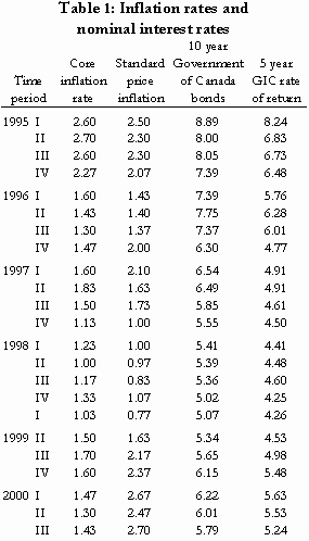
Table 1

Table 2 reports the real rates of interest obtained, first, from the real return bonds and, second, from adjusting the two nominal interest rates by each of the three measures of expected inflation. This produces seven measures of the real rate of interest.

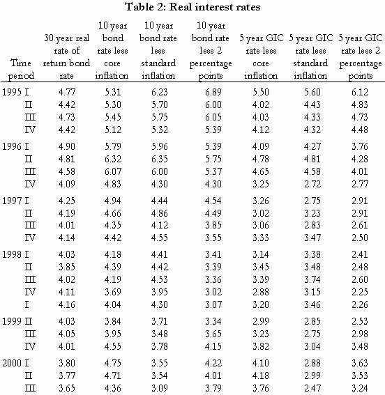
Table 2

What these figures suggest is, first, that the interest rate on real return bonds has been remarkably constant over the last three and a half years, rarely deviating very far from the 4.0 to 4.1 percent range until 2000, when it fell to approximately 3.7 percent.

Second, it is seen that the real rate of interest on 10-year government bonds has also fluctuated around 4.0 percent, but with far larger deviations than was seen with respect to the rate on real return bonds. Some of the wider of these deviations can easily be explained, however.

Note, for example, that the low real rates produced in 1998 and 1999 when the 2 percent inflation factor is used may have resulted because a long period of below-2 percent inflation had caused financial markets to believe that the Bank had lowered its target rate. (The conventional measure of inflation exceeded 2.0 percent only once between the first quarter of 1996 and the third quarter of 1999, when it was reported to be 2.1 percent in the first quarter of 1997.) If the markets had come to expect inflation rates of 1.5 percent in 1998 and 1999, for example, most of the real rates in those years would have been close to 4.0 percent.

The relatively high rates found in 2000 when long-run bond rates are discounted by core inflation, and the relatively low rates found in that year when they are discounted by the standard measure of inflation, could both be “explained” if it was found that financial markets had begun to accept the Bank of Canada’s statement that it was targeting a long-run inflation rate of 2 percent.

The consistently low rates found on GICs, however, are disconcerting. Over the entire period reported in Table 2, and for a number of years prior to that, the rates of return on GICs were significantly lower than those on government bonds. This suggests that plaintiffs would be extremely unwise to invest in GICs for the foreseeable future.

We conclude, therefore, that current estimates of the discount rate should be based on the rates observed on real return bonds and on long-term Government of Canada bonds. Arguably, these rates fluctuated around 4.0 percent for most of the last four years. They have, however, fallen slightly during 2000.

This raises the question of whether 2000 is an aberration, or whether the recent decline in real rates is the beginning of a long-term trend. Some evidence that the decline is expected to be short-lived comes from the Alberta government’s Budget 2000 documents. There, it is reported that nine respected forecasting agencies predicted an average interest rate on Government of Canada 10-year bonds of approximately 6.21 percent (over the years 2000-2003). As it is unlikely that those agencies would have forecast an inflation rate in excess of 2 percent, implicitly they have forecast a real rate of interest of approximately 4.1 percent.

In this light, we believe that a rate of 4.0 percent is the best, current estimate of long-run real interest rates. However, Economica will be monitoring movements in the interest rates on real return and 10-year Government bonds closely. If bond rates do not rise relative to the rate of inflation in the near future, we will be revising our real rate of interest forecast downward.

Christopher Bruce is the President of Economica and a Professor of Economics at the University of Calgary. He is also the author of Assessment of Personal Injury Damages (Butterworths, 2004).

Derek Aldridge is a consultant with Economica and has a Master of Arts degree (in economics) from the University of Victoria.

Scott Beesley is a consultant with Economica and has a Master of Arts degree (in economics) from the University of British Columbia.

Kelly Rathje is a consultant with Economica and has a Master of Arts degree (in economics) from the University of Calgary.

Combining Occupational Options

Posted on June 1, 2000March 24, 2017 By economica

by Christopher Bruce

This article was originally published in the Summer 2000 issue of the Expert Witness.

In many cases it is not clear at the time of trial what occupation the plaintiff would have entered had he or she not been injured, or what occupation he/she will now enter. In these cases, it is common for the vocational expert to offer a menu of possible occupations that are consistent with the plaintiff’s observed interests and aptitudes.

An issue that is crucial to the correct evaluation of damages in such cases, but which rarely receives the attention it deserves is: How should the incomes from the various occupations be “weighted” to determine an average, expected income for the plaintiff?

For example, assume that the vocational expert has concluded that, with appropriate upgrading, the plaintiff has the aptitude and skills to enter any one of three occupations – A, B, or C. Assume also that the following information is available about these occupations:

Annual incomes are:

A – $20,000
B – $25,000
C – $30,000

The number of employed workers in these occupations is:

A – 5,000
B – 1,000
C – 100

The unemployment rates in these occupations are:

A – 20%
B – 8%
C – 2%

The question is, how should the plaintiff’s expected income be calculated? I can think of four methods, each of which can easily be defended.

Simple Average

If the court has been provided with no information concerning which of these occupations the plaintiff will enter, it can be argued that, ex ante, there is an equal probability that he will enter each of them. Hence, each income should be weighted equally, producing an average of

($20,000 + $25,000 + $30,000)/3 = $25,000

Weight by Employment Opportunities

If it is assumed that the plaintiff will apply at random for jobs advertised in the newspaper, it is more likely that he will randomly “select” occupation A, with 5,000 jobs, than occupation B, with 1,000.

Alternatively, when the individual’s preferences are unknown, it can be argued that he is most likely to enter the occupations that other people have been observed to enter. Thus, as “most” individuals choose occupation A, it can be argued that it is more likely that the plaintiff will choose A than any other, all else being equal.

Recognising that there are 6,100 jobs in total, if income is weighted by employment opportunities, the average proves to be

[(5,000 x $20,000) + (1,000 x $25,000) + (100 x $30,000)]/6,100 = $20,984

Weight by Supply and Demand (Unemployment Rate)

If it is assumed that the plaintiff is more likely to be successful applying for jobs in which there are few applicants relative to the number of positions available, he is more likely to obtain a job at the occupations with the lowest unemployment rates. One method of allowing for this possibility is to weight the annual incomes by the inverse of their respective unemployment rates (that is by 1 minus the unemployment rate). These values are 80% for A, 92% for B, and 98% for C, with an average of 90%. Thus, relative to the average, the plaintiff is assumed to have a 0.889 (80/90) probability of finding a job at A, a 1.022 (92/90) probability of finding a job at B, and a 1.089 (98/90) probability of finding a job at C. In this case, the weighted average of the incomes in A, B, and C proves to be

(0.889 x $20,000 + 1.022 x $25,000 + 1.089 x $30,000)/3 = $25,333

Weight by Income

If it is assumed that the plaintiff is most likely to apply to the occupation with the highest income, the weightings change again. For example, if the probability that the individual will apply to each occupation is strictly proportional to the income earned in that occupation, the probability that he will apply to A is 80 percent of the probability that he will apply to B; and the probability that he will apply to C is 120 percent of the probability that he will apply to B. In this situation, the weighted average income will be

[(0.8 x $20,000) + (1.0 x $25,000) + (1.2 x $30,000)]/3 = $25,667

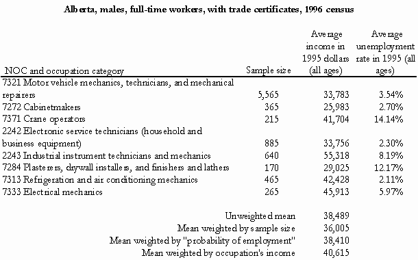
In the table below, I provide an example of these calculations drawn from a case in which Economica was involved recently. There it is seen that the vocational expert recommended eight possible occupations for the plaintiff. The average incomes for these occupations vary from $36,005 to $40,615, a difference of $4,610 per year, depending on which of the four averaging techniques is applied. If we assume that this individual was 25 years old at the time of the trial, an annual difference of $4,610 will alter the lifetime loss by approximately $100,000.

Clearly, it could prove crucial to determine which method is most appropriate. The first step is to speak to the vocational expert. Only if that expert indicated that the plaintiff was equally likely to enter each of the specified occupations would I consider it appropriate to employ the simple average method. If the expert has no opinion, my preference would be to weight the occupational incomes either by unemployment rate (to reflect supply and demand) or by numbers of employees (to reflect the likelihood that a plaintiff of known characteristics will choose a particular occupation). Weighting by income would only seem to be reasonable if the plaintiff was known to be particularly strongly motivated by financial considerations.

Table 1

Christopher Bruce is the President of Economica and a Professor of Economics at the University of Calgary. He is also the author of Assessment of Personal Injury Damages (Butterworths, 2004).

Case Comment: Madge v. Meyer

Posted on June 1, 2000April 20, 2017 By economica

by Scott Beesley

This article was originally published in the Summer 2000 issue of the Expert Witness.

In Madge v. Meyer, (Calgary Court of Queen’s Bench, 9601-01261, Judgment: December 31, 1999) Justice Brooker concluded that the plaintiff, Madge, had suffered a very serious head injury and would therefore be unable to operate his farm any longer. The plaintiff was assumed to be able to provide one third of his pre-accident value of work in the late pre-trial period and an average of 15 percent of that value in the future. (His abilities were expected to decline over time.) A farm expert assessed the pre-accident value of Mr. Madge’s work at $60,000 per annum in 1998 dollars. This loss of income calculation itself was a standard type of replacement cost analysis.

My comments on the case are related to Justice Brooker’s statement that

Madge’s situation presents the difficult issue of valuing a self-employed plaintiff’s loss of future income or work capacity when his business has not actually lost any income in the past nor seems likely to lose any in the near future due to his injuries (italics added).

This statement appears inconsistent with the evidence presented in this case to the effect that the plaintiff’s ability to continue in his previous capacity, as the manager of a large farm, was seriously compromised. In particular, it was clear that the management of the farm had been taken over by the plaintiff’s son, and that Mr. Madge’s contribution was now limited to part-time work at fairly menial tasks. Even for those tasks he had to be prompted by his wife and son. The evidence seems at odds with Justice Brooker’s comment that the business in which the plaintiff was the driving force had not lost any income.

Justice Brooker did go through the process of estimating the annual value of the plaintiff’s labour, and then deciding how much of that had been lost and would be lost in the future. I note, however, that Justice Brooker reached his final decision using the concept of loss of “income earning capacity,” (i.e. the loss of a capital asset), when that concept is really not necessary, or more accurately is redundant. When the courts ask economists to value the loss of earning capacity of an individual, the only method we have is to estimate what the annual figures would have been, and will be, and discount the difference back to the date of trial. The “capital asset” is valued by the present value of the stream of income that asset can produce.

The apparent lack of a loss at the level of the business in such situations usually simply means that family members or friends have assisted and were not fully paid, or paid at all, for those efforts. In addition it is possible (especially on a farm) that some long-term land or equipment maintenance, business development, or other work might simply not be done, with little apparent effect on immediate financial results. It seems likely that this is what has occurred in Madge. Even if Mr. Madge’s son had not been paid anything for his extensive assistance, the collateral benefit rule suggests that the loss should be assessed using the market value of any labour that replaced the plaintiff’s. The fact that no loss may have appeared at the corporate level is irrelevant. To suggest that there is no loss (as the defense apparently did in this case) because family members provided free labour to the plaintiff is in my view false. I presume that the defense would not argue directly that the son must provide such free labour indefinitely, and that the plaintiff’s future loss should be reduced by the value of that help. Yet that is what is implied whenever someone says “the business shows no loss and therefore the plaintiff has no loss.”

Note that if an injured party is provided with direct financial assistance from family members or friends, it is quite clear that that is a collateral benefit, and should be ignored in the loss calculations. (If the injured person then receives a damage award, it is possible they will repay the amounts provided, but whether or not they do so is irrelevant to the estimation of loss.) There is no reason to treat free labour any differently, yet it is common to hear the argument (or implication) that such assistance should: (A) benefit the defendant; and (B) be assumed to continue indefinitely. This false claim can only be made in the case of a self-employed plaintiff, who reports business income or has a corporation or partnership. The help provided by family and friends does not typically increase labour costs by much, if anything, and so the claim can be made that little or no change has occurred. Worse, the falsely reduced annual amount is then used to assess future loss. Another analogy can be found in household services losses. If an injured person is helped by a neighbour who cuts the lawn and shovels snow for a while, we would never reduce the household services claim by the value of that assistance. It would also be false to presume that the neighbour should provide that help until the injured party’s age 80 (when we typically end our household services loss calculations). Again, while we might expect the injured person to compensate the friend after settlement, that is a non-issue in the calculation.

This issue was addressed in an article in the Winter 1997 Expert Witness, in which Christopher Bruce and I discussed the D’Amato case. We noted that if the courts were to ignore the collateral benefit principle, and treat assistance freely given by friends and family as income (in D’Amato the issue was assistance in the form of overpayment from a business partner, and presumably friend), then not only would loss of income be severely underestimated, but the friends and family would be badly treated as well.

Imagine a plaintiff who cannot, for example, perform half of his previous work. His wife, who did not work at the time of the accident, begins to do that which he cannot, and takes no income from their jointly owned company (or takes the same amount she had been taking previously, if they had been income-splitting). If the wife’s work is identical in quality and there are no other losses (decreases in revenue, increases in costs), then the statements of the company are unchanged. The couple’s own personal tax returns would be unchanged as well. Yet it should be quite clear that the husband’s loss is half of his income. First, his earning capacity has been reduced by half; and, second, the apparent stability in his income has arisen only because his loss has been replaced with a collateral benefit – an altruistic “gift” from his wife. The presence of a collateral benefit should not, of course, reduce the estimated loss.

The problem is avoided with exact payments equal to the value of labour provided. Assume, for example, that the husband formerly received $80,000, and the wife did not work and received no income. After the accident she works and is paid $40,000, while his income falls by that same amount. The size of his loss of personal income is clear, even though there would be no change on their company’s financial statements. If the documentation was as simple as this, and the payments reflected the exact market value of each party’s labour, then the correct assessment would be easy. Unfortunately, this is rarely the case.

More realistically, assume that in the pre-accident case the wife had been receiving $20,000 per annum merely as an income-splitting measure. The husband’s reported income would have been $60,000. His labour actually had produced $80,000 in income, and now each of the spouses produces half of that. We would expect that their post-accident tax returns would report $40,000 each, simply because equal incomes are usually optimal for tax reduction. A shallow analysis would indicate that he had lost only $20,000 (= $60,000 – $40,000). Indeed, in an extreme case, the couple could still report the entire $80,000 on the husband’s return (there might be tax reasons to do so), and a cursory investigation would suggest that there was no loss.

There is really no substitute for actually estimating the share of company/family income that was due to the injured person’s labour, and then estimating how much of that has been lost. The fact that there may be little or no apparent change at the corporate, or even personal, level does not imply that no loss has occurred.

It bears repeating that if a proper analysis is not done, and the help provided by a friend or family member is mistakenly treated as income earned by the injured person, then a serious wrong could result. First, the person who provided the help might go uncompensated, since the plaintiff might not have the resources to pay them later. Second, the underestimation of the annual pre-trial loss could produce an extreme underestimation of the future loss. Oddly enough, in D’Amato, it appears that the Supreme Court correctly treated a large fraction of the plaintiff’s annual income as lost in the future, but did not compensate the partner for assistance provided in the pre-trial period. That decision essentially told partners (and family members and friends) that in helping an injured person you might not only be working for free, but you could also be undermining their loss of income case in doing so. Although D’Amato did receive full compensation for his future loss, it would appear that the overpayments made by his partner did cause an unjustified reduction in the pre-trial award. That uncompensated loss will be borne by D’Amato (if he pays back his partner), the partner (if he does not), or both of them. It would also seem to be quite possible that in other cases pre-trial and future losses will both be cut because of the failure to treat unpaid assistance as a collateral benefit.

At paragraph 175, Justice Brooker wrote “I cannot conclude that there has been an actual loss of farm profits to date.” He then stated shortly thereafter that “In my opinion, regardless of the profitability of the farm, Madge has suffered a loss of income or more accurately, income earning capacity for which he must be compensated.” Justice Brooker went on to note that Madge’s son should be entitled to more of the farm profits, since he had taken on “many of Madge’s work and responsibilities” since the accident. I would suggest that it would have been perfectly acceptable for the Justice to estimate the fraction of Mr. Madge’s work now done by his son and spouse (or not done at all!) and then presume that the annual loss is that fraction of his estimated annual income.

Note that if Madge had simply paid his son (and wife) exactly the amounts their additional labour had been worth, then his own personal income (or his business income, if the farm appeared as gross and net business income on his return) would have fallen by the precise amount of his loss. There are many reasons, however, why it is rare to have the loss appear in so clearcut a manner. First, the injured party simply may not have the money to pay a replacement, at least not in full. It is easy to say in hindsight that little help was paid for, so little could have been needed, but that is specious. The dollars which would have paid for replacement help are part or all of the plaintiff’s income, and in many cases the plaintiff can ill afford to give that up. That is exactly why friends and family will provide free or cheap assistance in many cases. Second, the assessment of what has changed as a consequence of injury can be complicated by issues like the income-splitting discussed earlier. Third, simply estimating labour income itself can be complicated, especially for farmers – some fraction of income is hidden, some is a return to capital employed, some is left in the business in any year while some is taken out. Depreciation taken could be more or less than the true economic loss of value of vehicles and equipment. Fourth, even just estimating what fraction of his or her former work the plaintiff can still do may not be easy. Fifth, one might only have financial information for a short period, containing years which are better or worse than a long-term average year. Sixth, the loss may not be fully valued unless things like long-term maintenance are considered (as mentioned earlier, are some things not being done which will create costs later?). Finally, any business analysis must separate changes caused by the plaintiff’s injuries from unrelated ones. If the business climate improved at roughly the time of the accident, it should be plain that that is not due to one person’s injuries, but I have seen a case treated that way.

Given the myriad difficulties associated with determining farm labour income precisely, and then estimating the fraction of income lost, I believe Justice Brooker’s approach to determining the loss in this case was reasonable. My purpose has been only to emphasize that that approach is not really in principle different from a standard assessment – it just uses an approximation for a hard-to-specify income figure. I also want to emphasize that to properly assess loss of income, the expert must consider the corporate and personal levels of tax, deal with the uncertainties listed above, and be sure not to treat freely given (or loaned!) assistance as income earned by the plaintiff.

Scott Beesley is a consultant with Economica and has a Master of Arts degree (in economics) from the University of British Columbia.

The Impact of Disability on Earnings: Results of the Health and Activity Limitation Survey

Posted on March 1, 2000March 24, 2017 By economica

by Christopher Bruce, Derek Aldridge, & Kris Aksomitis

This article was originally published in the Spring 2000 issue of the Expert Witness.

The 1991 Census of Canada contained two questions that asked whether respondents considered themselves to be “disabled.” Using the answers to this question (and the answers to a second, preliminary survey), Statistics Canada was able to create a file of approximately 34,000 individuals that it considered to be disabled. These individuals were then asked to complete a lengthy, detailed questionnaire, known as the Health and Activity Limitation Survey, or HALS. Another (approximately) 100,000 non-disabled individuals were asked to complete a less detailed questionnaire.

As the HALS questions concerned factors such as health, income, and education, it held great promise for use in personal injury litigation. Indeed, it is possibly the most extensive and reliable study of the disabled that has ever been conducted (not just in Canada, but worldwide). And one does see allusions to HALS data in many experts’ reports. But, for various statistical reasons, the data that have been released by Statistics Canada have proven to be less valuable than might have been hoped. As a result, to those of us working in the field of damage assessment, HALS has been a great disappointment.

Economica recently obtained a copy of the answers provided by each of the respondents to the HALS survey. From these data we have extracted a number of statistics that we believe will be of interest to the personal injury litigation community. Although we cannot hope to resolve all of the problems previously associated with HALS data in this short article, it is our expectation that the data presented here will, nevertheless, be of value.

Earnings

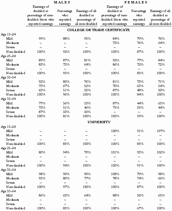
We have obtained earnings data for both males and females, divided into four age groups, four education levels, and four levels of severity of disability; that is, for 128 categories in total. (128 = 2 x 4 x 4 x 4). For each of these 128 categories we calculate three figures:

The average earnings of individuals in the category who had at least some earned income, as a percentage of the average earnings of non-disabled individuals in that age/sex/education category who had some earned income.
The percentage of individuals in the category who had some earned income.
The average earnings of all individuals in the category, as a percentage of the earnings of all non-disabled individuals in that age/sex/education category. (This category differs from the first because it includes individuals who reported no earnings.)

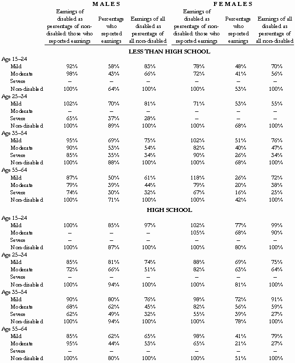
We present these data in Tables 1a & 1b (pages 5 & 6). Figures are shown for each of the four education levels: less than high school, high school, college or trade certificate, and university. As one would have expected, in each category earnings rise as one moves from non-disabled through mildly, moderately, and severely disabled. (We define “mild,” “moderate,” and “severe” disability in an Appendix to this article, thus allowing readers to determine to which of those categories individual plaintiffs belong.)

In virtually all categories, it is seen that the predicted effect that disability will have on earnings is lower if it is known that the individual will be working than if it is not known whether he or she will be able to work. That is, the earnings of the disabled are a higher percentage of the earnings of the non-disabled among the working population than they are among the total population. This is because a higher percentage of the disabled than the non-disabled earn no income.

For example, among males aged 35-44 with a high school education, those with a “moderate” disability earned 68 percent as much as the non-disabled if they earned anything at all. But 38 percent of the moderately disabled individuals in this age/sex/education group reported that they had no earnings, whereas only 6 percent of the non-disabled reported that they had no earnings. Thus, inclusion of those with zero earnings in the earnings figures had a much greater impact on the average earnings of the disabled group than similar inclusion had on the average earnings of the non-disabled. The result is that the earnings of all moderately disabled individuals in this group were only 45 percent of those of all non-disabled individuals.

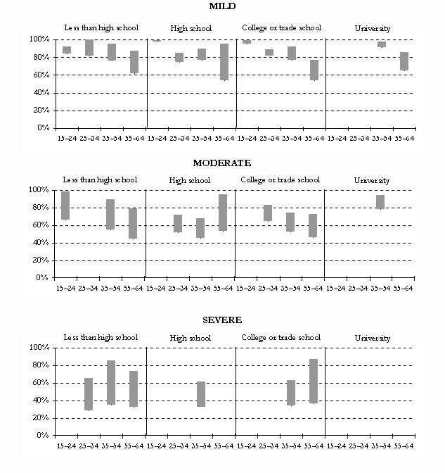
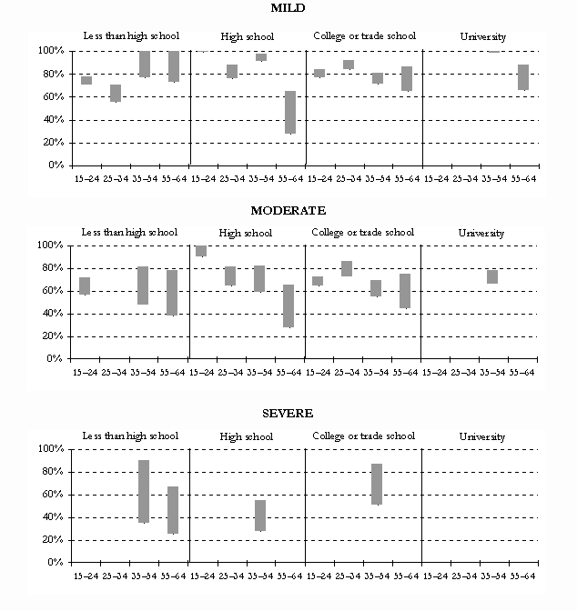
Charts 1a & 1b (pages 7 & 8) offer a graphical depiction of the data shown in the tables – and allow the reader to more easily observe the overall trend implied by the data.

Education

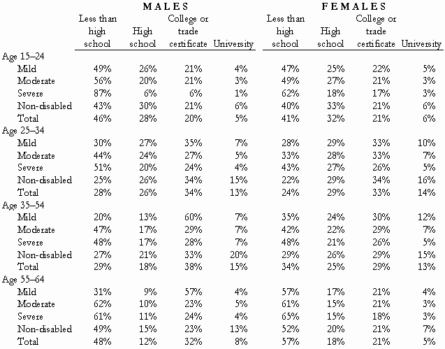
The earnings data reported in Tables 1a & 1b may underreport the effect of disability on earnings. The reason for this is that the disabled have lower education levels than do the non-disabled. If these lower levels result from the disability, then disability will have two effects: reducing earnings at each education level (Tables 1a & 1b) and reducing education levels.

In Table 2 (page 9), we report the distribution of education levels among the four categories of disability. It is seen in that Table that there is a higher percentage of university graduates among the non-disabled than among the disabled in every category; and a lower percentage of individuals who have not completed high school among the non-disabled than among the disabled in most categories. An interesting result is that mildly disabled males are much more likely than non-disabled males to have a college education or trade certificate. (However, this could occur if individuals with this level of education had a high probability of incurring injuries that caused mild disabilities.)

Conclusion

The tables and charts presented in this article suggest that the incomes of the disabled are lower than those of the non-disabled for at least three reasons: the disabled earn less when they work, even if they have the same levels of education as the non-disabled; the disabled are less likely to earn any income than the non-disabled; and the disabled have lower levels of education than do the non-disabled.

However, although the data presented here may be of some interest to personal injury litigants, the level of aggregation is so great that it seems unlikely that these data will be able to provide more than background information to the litigation process.

Appendix: Determination of the Degree of Disability

The purpose of this Appendix is to allow readers to determine whether Statistics Canada would classify a particular plaintiff’s disabilities as “mild,” “moderate,” or “severe.”

Statistics Canada asked 25 questions (see below), grouped into four categories. In the first category, the respondent was allocated a “score” of 0 if he or she answered “no,” a 1 if he/she answered “yes, but able,” and a 2 if he/she answered “yes, unable.” For example, the individual was allocated a 1 if he/she had difficulty hearing what was said in a conversation with one other person; and a 2 if he/she was unable to hear what was being said in such a conversation.

In the second category, the individuals were allocated a score of 1 if they answered “yes” to the question. (For example, “do you have difficulty with your ability to remember?”)

In the third category, individuals were shown a list of activities. If they were limited in their ability to engage in one of the activities they were allocated a score of 1; if they were limited in more than one of the activities they were allocated a score of 2.

Finally, individuals who had been diagnosed as legally blind received a score of 2.

The scores for all 25 questions were summed and individuals were allocated to the relevant levels of disability on the basis of their total scores. The scales used were:

LEVEL		RANGE
Mild		1-4
Moderate		5-10
Severe		11-43

It will be apparent that these are very imprecise categorisations. For example, using Statistics Canada’s scale, both an individual who was legally blind and an individual with a weak back would be categorised as “moderately” disabled, even though a reasonable a priori expectation is that those disabilities would affect individuals’ earning capacities quite differently. Similarly, both paraplegics and quadriplegics would be categorised as “severely” disabled, even though, again, we know that those disabilities have quite different effects on earnings.

I. In this category, individuals receive 1 each time they indicate that they have difficulty with the activity, but are able to undertake it (“yes, but able”); and 2 each time they indicate that they have difficulty with the activity and are unable to undertake that activity (“yes, unable”).

1. Do you have difficulty hearing what is said in a conversation with

1.1 One other person?

1.2 A group of at least three other people?

2. Do you have any difficulty seeing the following when you wear your ordinary glasses or contact lenses?

2.1 Newsprint?

2.2 The face of someone across a room?

3. Do you have any difficulty speaking and being understood?

4. Do you have any difficulty:

4.1 Walking 350 metres without resting?

4.2 Walking up and down a flight of stairs?

4.3 Carrying an object of 4.5 kg for 10 metres?

4.4 Moving from one room to another?

4.5 Standing for more than 20 minutes?

5. When standing, do you have any difficulty bending down and picking up an object from the floor (e.g. a shoe)?

6. Do you have any difficulty

6.1 Dressing and undressing yourself?

6.2 Getting in and out of bed?

6.3 Cutting your own toenails?

6.4 Using you fingers to grasp or handle (such as using scissors)?

6.5 Reaching in any direction (e.g. above your head)?

6.6 Cutting your own food?

II. In this category, the individual receives 1 if he or she responds “yes” and 0 if he/she responds “no.”

7. Are you unable to hear what is being said over the telephone?

8. Do you have ongoing difficulty with your ability to remember or learn?

9. Has a teacher or health professional ever told you or a family member that you have a learning disability?

10. In the past, persons who had some difficulty learning were often told they had a mental handicap or that they were developmentally delayed or mentally retarded. Has anyone ever used those words to describe you?

III. In this category, the individual receives 1 if he or she responds “yes” with respect to one of the categories; and 2 if he/she responds “yes” with respect to two or more categories.

11. Because of a long-term physical condition or health problem (i.e. one that is expected to last longer than 6 months) are you limited in the kind or amount of activity you can do

At home?
At school?
At work?
In other activities (e.g. travel)?

12. Because of a long-term emotional, psychological, nervous, or psychiatric condition, are you limited in the kind or amount of activity you can do

At home?
At school?
At work?
In other activities (e.g. travel)?

13. Do you feel limited by the fact that a health professional has labelled you with a specific mental health condition, whether you agree with this label or not?

At home?
At school?
At work?
In other activities (e.g. travel)?

IV. Finally, if the individual had been diagnosed as legally blind, he/she was given a score of 2.

14. Have you been diagnosed by a specialist as being legally blind?

Table 1a: Earnings of disabled individuals compared to earnings of non-disabled individuals

Table 1a

Note: A dash indicates that the category’s sample size is too small to report a statistically reliable estimate.

Table 1b: Earnings of disabled individuals compared to earnings of non-disabled individuals

Table 1b

Note: A dash indicates that the category’s sample size is too small to report a statistically reliable estimate.

Chart 1a: Earnings of disabled males compared to earnings of non-disabled males

Chart 1a

Note: This chart graphically depicts the data shown in Tables 1a and 1b. The top of each bar represents the earnings of disabled males who reported earnings as a percentage of non-disabled males who reported earnings. The bottom of each bar represents the earnings of all disabled males (whether they reported earnings or not) as a percentage of all non-disabled males (whether they reported earnings or not). Where no bar is shown indicates that the category’s sample size is too small to allow us to report an estimate (corresponding to the dash in Tables 1a and 1b).

Chart 1b: Earnings of disabled females compared to earnings of non-disabled females

Chart 1b

Note: This chart graphically depicts the data shown in Tables 1a and 1b. The top of each bar represents the earnings of disabled females who reported earnings as a percentage of non-disabled females who reported earnings. The bottom of each bar represents the earnings of all disabled females (whether they reported earnings or not) as a percentage of all non-disabled females (whether they reported earnings or not). Where no bar is shown indicates that the category’s sample size is too small to allow us to report an estimate (corresponding to the dash in Tables 1a and 1b).

Table 2: The distribution of education levels among the four categories of disability

Table 2

Christopher Bruce is the President of Economica and a Professor of Economics at the University of Calgary. He is also the author of Assessment of Personal Injury Damages (Butterworths, 2004).

Derek Aldridge is a consultant with Economica and has a Master of Arts degree (in economics) from the University of Victoria.

Kris Aksomitis was a research associate with Economica and an MA student in Economics at the University of Calgary.

Economica

Assessment of damages in personal injury and fatal accident litigation

Year: 2000

Assessment of damages in personal injury and fatal accident litigation

Contents:

Data

Comparisons

Econometric modelling

1. Introduction

2. Alternative methods of calculating the impact of reduced life expectancy

3. An Example

4. Comparison of the methods

5. Conclusion

Contents:

Real versus nominal interest rates

Alternative measures of the interest rate

Estimating the rate of inflation

The data

Contents:

Simple Average

Weight by Employment Opportunities

Weight by Supply and Demand (Unemployment Rate)

Weight by Income

Contents:

Earnings

Education

Conclusion

Appendix: Determination of the Degree of Disability