by Christopher Bruce

On January 1, 2004 the federal Personal Information Protection and Electronic Documents Act was extended to every organization that collects, uses or discloses personal information in the course of a commercial activity within a province. On the same date Alberta’s Personal Information Protection Act came into effect. The purpose of the (Alberta) Act is to “govern the collection, use and disclosure of personal information by organizations” (see www.psp.gov.ab.ca/faq.html). In light of these events, we outline Economica’s privacy policy:

• We do not reveal any information concerning the specifics of any case, including the names and personal circumstances of the litigants, to any party other than the law firm that has retained us – unless that firm has specifically requested that we do so. We will not, for example, provide copies of our reports to the plaintiff or defendant, to any other expert who has been retained in the litigation at hand, or to any other law firm that is involved in the litigation without a specific request by the firm that has retained us.
• All of the documents that we receive concerning the specifics of a case are kept in secure areas and/or in secure computer files. All such documents will be maintained in such a manner that they are not accessible to casual observation by visitors to our offices.
• We will not discuss a case with any party other than the firm that has retained us, without previously having received the permission of that firm. We will not, for example, request personal information from the plaintiff, the plaintiff’s family, or the plaintiff’s employer, or from other experts without first informing the firm that retained us.
• When speaking with third parties, such as employers, we will not reveal the name or circumstances of the plaintiff unless it is necessary to do so. If, for example, it is possible to obtain details concerning the plaintiff’s pension plan from his/her employer without revealing the plaintiff’s name, we will do so.
• When disposing of confidential files concerning any litigant, we will have those files shredded by a professional firm.

Christopher Bruce is the President of Economica and a Professor of Economics at the University of Calgary. He is also the author of Assessment of Personal Injury Damages (Butterworths, 2004).

by Christopher Bruce

According to the most recent Statistics Canada data, automobile insurance premiums in Alberta increased by 68.6 percent between 2001 and 2003 (29.9 percent per year), at a time when the consumer price index increased by only 8.0 percent (3.9 percent per year). Similarly, over the 10-year period 1994-2003, premiums increased by 97.8 percent (7.9 percent per year) while the consumer price index increased by only 26.4 percent (2.6 percent per year). (See Figure 1.)

Although the government has reacted to this increase by introducing wide-ranging legislative changes, no satisfactory explanation has been given for why premiums should have risen so dramatically. The purpose of this article is (i) to review eleven of the explanations that have been given for rising premiums and (ii) to investigate those explanations to determine whether they are consistent with the evidence.

1. Number of accidents

Everything else being equal, an increase in the number of accidents per driver must increase insurance companies’ average payouts and, therefore, their average premiums. However, statistics indicate that the number of accidents has not increased significantly in the last decade. Between 1994 and 2001, for example, the number of collisions increased only from 431.4 to 460.5 per 10,000 vehicles, an average rate of increase of less than one percent per year. This cannot explain the sizeable premium increases of the last few years.

2. Severity of accidents

Even if the number of accidents had declined, the costs of claims per driver might have increased if the average severity of accidents had risen. If fewer people had been injured than in the past, but each injury had been much more serious than previously, total costs of claims might have risen.

With respect to severity, it is known that whereas the number of collisions involving injuries or fatalities increased only slightly between 1994 and 2001 – from 72 to 83 per 10,000 registered vehicles – and the number of collisions involving property damage remained almost constant – at about 360 per 10,000 registered vehicles – the number of “bodily injury” claims almost doubled – from 65 to 112 per 10,000 registered vehicles – over the same period. As bodily injury claims are generally much more expensive than other types, this trend suggests that the average cost of claims should have risen over the 1994-2001 period. Indeed, the Insurance Bureau reports that the average cost of injury claims rose by 44.6 percent (4.2 percent per year) between 1993 and 2002.

What these statistics do not explain, however, is why automobile insurance premiums increased so dramatically in 2002 and 2003. The statistics indicate that whereas the dramatic rise in premiums has been a recent phenomenon, the number and severity of bodily injury claims per vehicle has increased steadily for almost ten years. This evidence suggests that the recent rise in premiums is not closely connected with the increase in severity of accidents.

3. Damages

Even if the number and severity of accidents had remained constant, it is possible that the average cost of accidents could have risen if the courts had become more liberal in their awards of damages to accident victims. With respect to serious personal injury and fatal accident claims, the evidence on this question is clear, however – in the last 20 years there has been virtually no change in the manner in which the courts assess damages. Although there are no definitive statistics on this issue, the principles of damage assessment, in major injury cases, have not changed in Alberta since the mid-1980s. If damages for major injury cases have increased, it is not because there has been a change in the attitude of the courts; it is because Albertans’ incomes have been rising – necessitating larger awards to compensate victims for their losses of income.

It is possible that damage awards for minor injuries have increased substantially. However, it is noteworthy that insurance companies, who have argued that this is one of the major causes of increased premiums, have not released any data to back this claim. It seems reasonable to draw an adverse inference from this failure. Surely if the data supported the insurance industry’s arguments, they would have made those data public.

4. Fraud

Insurance companies commonly argue that consumer fraud is a major source of inflationary pressure on insurance rates. There are two major problems with this argument. First, although insurance fraud undoubtedly occurs, insurance companies have been unable to provide any statistically reliable evidence to show that fraudulent claims amount to more than a small percentage of payouts.

Second, and more importantly, even if fraud was a major problem, no evidence has been put forward to suggest that fraudulent claims have increased substantially in the last two years. For an increase in fraud to explain a significant portion of the 69 percent increase in premiums that has been observed, fraudulent claims would have to have increased dramatically. There is no evidence at all that this has occurred.

5. Medical costs

A recent study by the Insurance Research Council (a U.S.-based agency) found that “escalating medical costs are the key factor behind” the growth in automobile insurance claims in the past five years. It seems unlikely that this source could account for a significant portion of the recent rise in premiums in Alberta, however, as a substantial portion of medical costs resulting from automobile accidents are covered by Alberta Health Care. Since 1996, those costs have been covered under an annual levy that has increased at a relatively steady rate, of approximately 12 percent per year. For this source to explain a significant portion of the 69 percent increase in premiums seen in the last two years, there would have to have been a dramatic increase in the annual levy, an increase that has not been observed.

6. Legal costs

An additional component of the cost of insurance is the fees charged by lawyers and other experts. Although a substantial portion of victims’ legal fees are paid by the victims out of their damages – and, therefore, do not contribute to insurance companies’ costs – insurers have to hire their own lawyers and may sometimes have to pay a portion of the victims’ legal fees. Nevertheless, any argument that these costs have contributed to the substantial increase that has been observed in automobile insurance premiums founders on a lack of evidence that these fees have increased substantially in the last few years. It is one thing to argue that legal fees may, or may not, be “too high,” it is another thing altogether to argue that they have risen as a percentage of insurance costs.

7. Return on investment

To a certain extent the costs of operating an insurance company are offset by the company’s ability to invest the premiums it has received until drivers make their claims. The higher is the interest on those investments, the less does the company have to charge in the form of premiums. Some commentators have argued recently that the observed increase in premium costs has resulted from the decline in the average rate of return on investments.

This is not a compelling argument, however, as this decline cannot explain more than a small portion of the dramatic increases in premiums. If insurance companies hold premiums for half a year on average (that is, if premiums are collected at the beginning of the year and then spent at a constant rate over the year), and if the rate of return on investments is, say, 8 percent, then the interest that is collected will (on an annual basis) equal 4 percent of premiums. If the rate of return then declines to 5 percent, the effective return on the investment of premiums will fall to 2.5 percent, a drop of only 1.5 percent. As this is roughly the order of magnitude of recent declines in rates of return, this factor cannot explain a significant percentage of the recent increases in premiums.

8. Administrative costs

Approximately 25 to 30 percent of an insurance company’s costs are for administration – salaries of salespeople and adjusters, rent, cost of supplies, advertising expenses, etc. There is no evidence to suggest that these costs have risen significantly in the last few years.

9. Re-insurance

Insurance companies have argued that one of the most important sources of increased costs in the last two years has been the increase in premiums that they have had to pay to re-insurance companies since September 11, 2001. This argument is implausible. Figure 1 illustrates the increases in both automobile and homeowners’ insurance premiums in Alberta in recent years. If re-insurers had raised their rates in response to the perceived increase in terrorism, they would have raised those rates by at least as much for homeowners’ insurance as for automobile insurance. But it is seen clearly in Figure 1 that homeowners’ insurance premiums rose by far less than did automobile insurance premiums. This provides compelling evidence that increases in re-insurance premiums have not been a major source of the reported increase in automobile insurance premiums.

10. Collusion

Some critics of the insurance industry have argued that the recent increases in automobile insurance premiums have resulted from collusive behaviour among insurance companies. This argument is suspect for two reasons. First, it is difficult to explain why insurance companies would have raised premiums for automobile insurance and not for homeowners insurance. Second, there are more than 100 automobile insurance companies operating in Alberta. Over a century of experience suggests that it is extremely difficult even for an industry of only three or four firms to maintain a collusive stance. It is unlikely that 100 firms could do so.

11. Statistical interpretation

There is some concern that the dramatic increases that have been observed in automobile insurance premiums in the last few years have resulted from the way that statistics are collected and reported rather than from “real,” underlying factors. Two arguments have been made in this respect.

First, the Insurance Bureau argues that the manner in which Statistics Canada collects information about automobile insurance premiums produces misleading results. Nevertheless, the Bureau’s own data (published in the December 2003 issue of their newsletter Perspective) indicate that automobile insurance premiums in Alberta rose by approximately 63 percent (5 percent per year) between 1993 and 2003 and by approximately 30 percent (14 percent per year) between 2001 and 2003. Although these numbers are much lower than those produced by Statistics Canada, they are still substantially higher than the overall consumer price inflation figures for those periods. (Also, whereas Statistics Canada’s data measure changes in the price of a fixed “basket” of insurance policies, the IBC data measure changes in the costs of actual insurance policies that have been purchased. Thus, if, as premiums rise, consumers purchase less comprehensive policies, the IBC data will underestimate the rate of increase of given policies.)

Second, it is well known to observers of the automobile insurance industry that premiums move in a cyclical manner. When premiums are relatively low, insurers’ profits fall and many firms leave the market. This reduces competition and allows premiums to rise. But as that happens, profits also rise, attracting new firms, and driving down premiums again. Typically, this cycle takes approximately 10 years. The data in Figure 1 show, for example, that there were significant increases in premiums in the early 1980s, early 1990s, and early 2000s; and stagnation of premiums in the mid-1980s and mid-1990s.

This observation suggests that the recent, dramatic increases are simply part of a larger, cyclical movement in automobile premiums. Even if this is true, however, the average increase over the last 10 years – even when calculated on the basis of the IBC figures (5 percent per year) – has been more than double the average rate of consumer price inflation. Clearly, cyclical and statistical factors alone cannot account for this substantial increase.

Conclusion

The information that has been reviewed in this paper suggests that two factors are primarily responsible for the pattern of premium changes that have been observed in Alberta in the last decade. First, the dramatic increases in the last two years represent a “natural” upturn in a long term cycle in premiums. Past patterns suggest that these increases will be followed by stagnation of premiums for the next six or seven years.

Second, there is some evidence to suggest that the average severity of personal injury claims has been rising. As I find no evidence that this increase has been due to fraud, to an increase in the number of accidents, or to changes in the criteria employed by the courts to calculate damages, it appears that the most plausible explanation is that the losses suffered by plaintiffs have been increasing in value.

A large number of individuals were kind enough to provide me with assistance in the preparation of this article. I would particularly like to thank Don Higa, Jim Rivait, Walter Kubitz, Derek Aldridge, and Harris Hanson.

Christopher Bruce is the President of Economica and a Professor of Economics at the University of Calgary. He is also the author of Assessment of Personal Injury Damages (Butterworths, 2004).

by Christopher Bruce

In the first article in this newsletter, I analyzed the arguments concerning eleven possible sources of increased automobile insurance premiums. The purpose of this article will be to review each of those sources to determine whether there are changes in government policy that might reduce premium costs.

1. Number of accidents – Experience Rating.

The Alberta government has already taken one of the boldest and most innovative steps possible towards reducing the number of automobile accidents. This is their proposal to introduce experience rating – the direct tying of premium values to drivers’ accident-causing behaviour – to the automobile insurance sector.

Experience rating has two highly desirable characteristics. First, the individual driver has complete control over his or her premiums. If individuals drive cautiously, avoiding accidents and driving violations, their premiums will decline to the lowest available rate. Furthermore, individual drivers’ rates will not be relatively high just because they happen to belong to a group, like young males, that has a relatively high accident rate.

Second, there is a substantial body of statistical evidence to show that when insurance premiums are related to experience, accident rates fall. When individuals know that they can reduce their premiums significantly by driving more carefully, they do so.

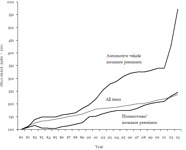
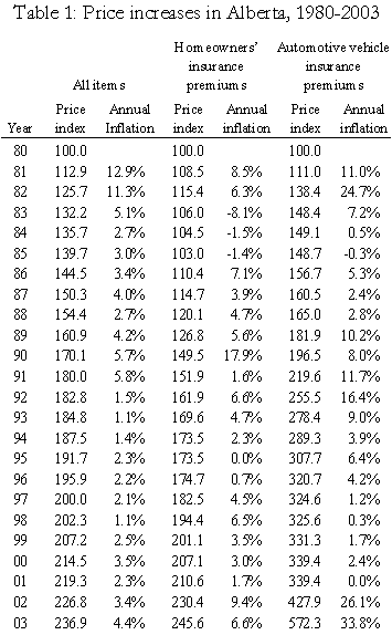
Under the government’s proposal, the impact of a serious driving offence or an at-fault accident will be much greater than it is currently, under what is known as “actuarial” rating of premiums. For example, under the proposed system, a typical Edmonton driver who has recently begun to drive (i.e. who has no “experience”) will pay a premium of about $2,000. After four years of no accidents or driving offences, that driver will pay only $700 – a saving that will continue for each and every year into the future as long as the driver has no accidents or convictions. One would expect an annual saving of $1,300 to be of sufficient size that it would induce most individuals to take additional precautions against unsafe driving.

Furthermore, the proposed system would move the driver four steps up “the premium ladder” each time he or she had an at-fault accident. So the driver with four years of accident free driving would be bumped from the reduced $700 premium to the $2,000 base premium, losing the entire $1,300 “bonus”.

And the incentive to avoid driving convictions is even stronger. A single impaired driving conviction would increase premiums by 200 percent.

These proposals are highly desirable. The government deserves far more credit than it has received for recommending them. Nevertheless, the government needs to reconsider two aspects of its plan.

First, it is mistaken in its proposal that a government agency should set the base premium rate. For example, in the case discussed above, the $2,000 base premium for Edmonton drivers was not one chosen by the insurance companies, but by the government. This is unreasonable for two reasons. First, the government cannot know what the true cost is to the insurance companies of providing insurance. As a result, the base rate that it will choose is almost certain to be either too high or too low.

If it is too high, insurers will make excess profits at the expense of Alberta drivers. If it is too low, insurance companies will make losses and some of them will refuse to provide coverage to Albertans.

Second, when the government sets premiums, the competitive incentive for insurance companies to find ways to lower rates is lost. If insurance companies are forced to charge the same rates regardless of how efficient they are, there is less incentive for them to seek ways of being efficient. It is these competitive pressures that keep premiums from rising more than they have.

There is a simple solution to these problems: the government should set only the percentage increases and decreases that are to result from various “experiences” and leave the insurers to set the base rates from which those increases and decreases are to be calculated. This will get the government out of the business of setting rates, while leaving intact the strong incentives created by a system of experience rating.

The second problem with the new legislation is that it does not deal with the adverse incentives that it gives to insurance companies. Specifically, experience rating results in a situation in which insurers know they will make substantial profits on some classes of customers and lose money on others. Thus, it gives them a strong incentive to refuse to insure the money-losing group. In the scheme proposed by the Renner committee, that group will be composed primarily of young males.

Insurers will lose money on this group because the number of accidents drivers have had in the past is only loosely related to the number that they can be expected to have in the future. What decades of statistics tell us is that a nineteen-year-old male with a perfect, three-year driving record is more likely to have an accident in the next year than is a forty-year-old male with the same driving record. And a nineteen-year-old who had an accident last year is more likely to have an accident next year than is a forty-year-old with the same experience. This means that insurers will expect to pay out more claims to nineteen-year-old drivers than to forty-year-old drivers.

Assume, for example, that ten percent of nineteen-year-old drivers who have had a clean record for three years will have an accident in the next year; whereas only five percent of forty-year-olds with a similar record will have an accident next year. If the average accident costs the insurance company $10,000, it will expect to pay out an average of $1,000 for each nineteen-year-old and $500 for each forty-year-old.

If the government forces insurers to charge the two groups the same premium, they will have to charge something between $500 and $1,000 just to cover their expected claims costs. For example, if the two groups were the same size, the premium would be $750 (the average across the two). But this means that they will expect to make a $250 profit on the average driver in the older group and a $250 loss on the average driver in the younger group.

As insurance companies are profit-driven, we can expect that they will respond by doing their best to attract older drivers – and to turn away younger drivers. The stakes are high. Those companies that find themselves with a relatively high percentage of young drivers will lose money and will soon be forced out of the market. Companies will use every loophole at their disposal to attract as many drivers in the older age groups as possible.

For example, companies might offer to sell automobile insurance through employers, in much the same way they currently sell long-term disability and dental plans. As employees are predominantly in the 25-64 year age group, and as high risk drivers are predominantly in the 16-24 and 65+ age groups, such a practice would allow firms to “skim” off the low-claim drivers.

The government will need to introduce strict controls to ensure that companies are not seriously disadvantaged if they write insurance for groups whose average claims exceed average costs.

2. Severity of accidents – Improved policing.

Reductions in severity are most likely to come from improvements in the design of automobiles; and in the use of safety devices such as seat belts and air bags. Nevertheless, provincial governments can reduce severity by enforcing highway speed limits more strictly – particularly on segments of roads that are known to have high accident rates.

Recent scientific evidence, published in journals such as Accident Analysis and Prevention, Injury Prevention, and the Canadian Medical Association Journal, concludes that the two changes that offer the greatest promise for reducing the incidence and severity of accidents are: first, raising the legal drinking age; and, second, banning the use of hand-held cellular telephones by drivers of moving vehicles.

3. Damages – Restrictions on tort.

Many of the proposals that have circulated in the last year or so have had to do with the placement of restrictions on tort damages. In general, these proposals are based on the assumption that victims are currently being “overcompensated;” hence, a reduction in damages will not cause a hardship to victims. The two most commonly-made proposals are that individuals should not be able to claim from two insurers for the same loss – the “double compensation” issue – and that loss of income should be calculated net of income taxes – because victims do not have to pay taxes on their awards, they will be adequately compensated if damages are based on after-tax income.

Typically, double compensation occurs when the victim is compensated for loss of income both by the defendant and by the victim’s own long-term disability insurance. Under the new legislation in Alberta, victims will be allowed to collect from only one of these parties. This proposal seems reasonable except that it is usually suggested that the victim be required to collect from his or her own insurance company. Effectively this requires that the victim be made to pay for damages caused by a negligent driver – and it allows the negligent driver to evade responsibility for his/her actions. Neither of these outcomes seems defensible. Furthermore, if disability insurers are able to re-write their policies in such a way as to avoid paying damages when their clients are able to collect from negligent drivers, the legislation will affect only disability insurance premiums (which will decrease), not automobile insurance premiums.

The second proposal for reducing tort damages – that victims be compensated only for after-tax losses – also seems reasonable. As plaintiffs do not pay taxes on court-awarded damages, the payment of “gross” income overcompensates them. The primary argument against this proposal is that plaintiffs currently rely on this “overcompensation” to help them pay for their legal fees (which are only partially paid by the defendant). If plaintiffs have to pay for their legal fees out of after-tax income, their awards net of legal fees will leave them undercompensated.

A third element of the new legislation sets limits on the award of “non-pecuniary” damages. This is not based on the assertion that victims are being overcompensated by the courts. Rather, it is based on the assertion that victims of “minor” injuries are exaggerating their injuries and, therefore, defrauding the system. The issue of fraud is discussed in the next section.

4. Fraud.

Setting limits on damages is an entirely inappropriate method of dealing with fraudulent claims, primarily because it punishes the innocent. If fraud is an important factor in the determination of automobile insurance premiums, there are two appropriate responses. Insurers can increase their vigilance; and, in cases of egregious behaviour, they can ask the government to lay criminal charges. As both of these responses are already available to the insurance industry, the government does not need to take further steps.

5. Medical costs.

It is clear that public policy towards medical costs is unlikely to be influenced significantly by government concern over automobile insurance premiums. In this area, drivers and insurers can only hope that government health policy incidentally acts to reduce personal injury claims costs.

6. Legal costs – no fault.

It is often argued that legal costs could be minimized if a form of no fault insurance was introduced. Whatever the advantages of no fault might be, there are three important problems with it that must be dealt with before such a proposal can be considered seriously.

First, because more parties can make claims in a no fault system than in a fault system (“at fault” drivers can make claims in no fault systems but not in fault systems), there is very little chance that no fault will reduce premiums. Indeed, the evidence shows that no fault jurisdictions have premiums very similar to those in fault jurisdictions.

Second, the purported source of savings in a no fault system is that accident victims are denied access to the court system; hence legal bills are reduced. But, the courts serve an important function – they allow parties to appeal decisions made by their insurance companies that they feel are unfair. It is possible that an appeal system can be introduced to no-fault insurance, but there is some evidence to suggest that if such a system really is fair, it will cost as much as do the courts. In short, any savings in administrative costs tend to come at the expense of justice.

Third, there is consistent, strong evidence to suggest that there are more accidents in no fault jurisdictions than in fault jurisdictions because drivers in the former do not have to take responsibility for their actions. (Recent statistical studies conclude that when no fault insurance is introduced, the accident rate rises by approximately 6 percent.) Indeed, not only are the drivers who are at fault for their own injuries not made to pay higher premiums, they are fully compensated by the insurance system for any costs they incur.

7. Return on investment.

If insurance companies have been harmed by falling rates of return on their investments, there is nothing the government can do to help, short of making short-term loans at below-market rates.

8. Administrative costs – Public insurance.

It has often been suggested that administrative costs could be reduced if the private insurance system was replaced by a government-run monopoly. This suggestion ignores the fact that monopolies have been found, almost universally, (i) to be less responsive to their customers than are competitive firms; and (ii) to be less efficient than are firms that have to face competitive pressures. (Some proponents suggest that automobile insurance is less expensive in Saskatchewan and Manitoba than in Alberta because it is provided by monopoly in the former two provinces. However, this ignores the many subsidies that those insurers receive from their governments and also ignores the fact that British Columbia’s premiums are not significantly different from Alberta’s.)

9. Re-insurance.

Following the terrorist attacks of September 11, 2001, re-insurance companies have raised their premiums significantly. As the terrorist attacks should have only a negligible effect on automobile insurance claims, the re-insurers’ actions are unjustifiable. It might be appropriate for the Government of Alberta to provide re-insurance coverage to firms working within Alberta until re-insurance rates return to a level that is consistent with the risk that is being faced.

10. Collusion.

Unless some evidence is presented to suggest that automobile insurers are colluding, no action needs to be taken on this issue.

11. Statistics.

If Statistics Canada has overestimated the rate of increase of automobile insurance premiums and if premiums do follow a regular cycle, which is currently at its peak, then there is little or no rationale for the Alberta government to do anything about premiums. Alberta might cooperate with the Insurance Bureau and Statistics Canada in reassessing the method by which premium inflation is measured; but, otherwise, Alberta merely needs to wait a year or two and that inflation rate will fall significantly by itself. The drastic changes proposed by the government are completely out of line with the (non) seriousness of the situation.

Summary

This article has concluded that the government would be justified in adopting the following policy changes:

• Introduce experience rating, as proposed by the Renner committee, but without government control over the base premium rate.
• Increase police surveillance of moving traffic violations, particularly in areas identified as being of high risk.
• Raise the legal drinking age.
• Ban the use of hand-held cellular telephones by drivers of moving vehicles.
• Introduce a regulation that losses of income be made on an after-tax basis.
• Provide re-insurance to the automobile insurance industry until rates return to a level that can be justified based on expected claims.
• Cooperate with Statistics Canada and the Insurance Bureau of Canada in investigating the manner in which the inflation rate of automobile insurance premiums is measured.

Christopher Bruce is the President of Economica and a Professor of Economics at the University of Calgary. He is also the author of Assessment of Personal Injury Damages (Butterworths, 2004).