ACTLA Presentation – Loss of Income for Self-Employed Plaintiffs

Derek Aldridge, Economica

derek@economica.ca

(I consent to redistribution of this unmodified document)

ACTLA Presentation – Lunch and Learn

March 25, 2021

Loss of income for self-employed plaintiffs

I will briefly discuss the approach that I use to estimate the loss of income for self-employed plaintiffs. Simply determining the true income of a self-employed worker can be challenging, and I will address some of these challenges. I will also discuss some approaches that can be used to estimate their loss of income.

Note that my tables and charts are based on actual cases I have worked on, but I have made various adjustments to simplify the presentation to preserve confidentiality.

Estimating the income of a self-employed worker

Determining the income of a self-employed worker can be much more complicated than for a regular employee.

For a plaintiff who is an employee and not self-employed, their income is simply the amount they are paid by their employer. Employment insurance income is also relevant for our calculations. Both of these sources of income are usually easy to determine by looking at the plaintiff’s income tax records. An employee might have income tax records that look something like this:

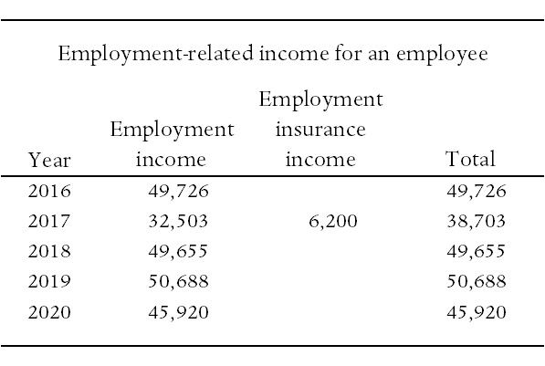
Usually, the income tax records will give us an accurate description of the income of an employee-plaintiff – at least for the pre- accident period. After the accident there can be income replacement benefits that do not appear in the income tax records.

For a self-employed worker, their personal income tax records usually only tell us part of the story of their income. The personal income tax records for a self-employed plaintiff might look something like this:

For the self-employed worker, the income reported on their personal tax returns will often not reflect their true income in each year. I will discuss this below.

For my purposes, there are two categories of self-employed workers: those who operate their business as a sole proprietorship, and those who operate a corporation.

Sole proprietorship

  • These are usually fairly straightforward.
  • All business income appears on the personal income tax returns – usually as gross and net business income.
  • There is a statement of earnings with the personal tax return that shows a detailed description of revenue and expenses.
  • All business income is paid to the business owner each year. There is no separate corporation where profit can be held separately from the owner. Because there is not a separate corporation, most of the information we need to estimate the plaintiff’s income is usually contained in their personal tax records.

Corporation

  • These are more complicated, and I will focus my discussion on cases when the plaintiff’s business is a corporation.
  • The plaintiff operates his business through a numbered or named corporation (for example, 1234567 Alberta Ltd, or Derek Aldridge Consulting Ltd). The corporation is a separate entity from the plaintiff, so income earned through the corporation will not necessarily appear on the plaintiff’s personal income tax records. That is why we need the corporate financial statements.
  • The business income statements show the revenue and expenses for each year. When I combine the income statements for several years, I create a table that looks something like this:

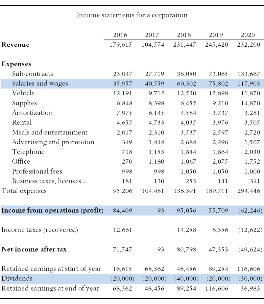
The income statements can get quite complicated, but in general, we see the revenue at the top, which is the income the business earned each year. Then we have various categories of expenses. The business owner usually pays himself a salary, and it is included here as an expense, because his salary is an expense to the business. The salary for other workers at the business is also likely included in that same expense category. The revenue less the expenses gives us the income from operations (profit), before accounting for corporate taxes. In principle, the business owner could pay himself a high enough salary so zero profit would remain. But usually what happens is some of the profit is left in the business as retained earnings, which is effectively savings (the corporation does not need to pay out all profit to the owner every year). The business financial records will show us how these retained earnings have accumulated over time, and will also show us when the owner draws down these savings by taking dividends.

When examining the corporate income statements, I am most interested in how much the business paid the owner in salary (part of the business expenses), and how much before-tax profit the business had after expenses, since that profit effectively belongs to the owner and could have been paid to him as part of his salary. The business owner’s income is the total of the salary (employment income) that the business paid him, plus the profit that the business earned. The salary is reported on his personal tax return, but the business profit is not. The owner might also report dividend income from the corporation, but I do not normally count this as part of his income. Because I am attributing all of the business profit to the owner in each year, this captures all of the dividend income that could be paid in future years.

Note that dividend income can cause some confusion because it does not necessarily reflect earnings from the year under consideration. If the business has accumulated significant retained earnings from previous years’ profits, the owner could still pay himself a large dividend in a year when business was poor.

Below I compare the income reported on this business owner’s personal income tax records with his true income:

We see that there can be quite a large difference between the business owner’s true income and the income that is reported on his personal income tax records. Another potential complication is that the corporation reports its income in a fiscal year, which may be different from a normal calendar year. So if fiscal 2019 for the corporation is the 12-month period from August 2018 through July 2019, it will make it more difficult to match up income reported on the personal tax returns with the corporate financial statements.

Documents and information required

Below I list some of the documents and information that I like to have when dealing with a self-employed plaintiff.

  • The business income statements show the revenue and expenses for each year.
  • The balance sheet is usually included with the income statement as part of the annual financial statements that are usually prepared by an accountant. However, there is usually not much useful for me in the balance sheet.
  • I need the plaintiff’s personal income tax records because they will show the salary (employment income) that he drew from the business.
  • Sometimes the business pays a salary to another family member. Perhaps the owner’s wife does bookkeeping and the business pays her a salary of $20,000 per year. That’s fine, but if she is being overpaid for this work (income-splitting) then I should account for this. For example, if she is being paid $20,000 but an arms-length bookkeeper would only be paid $12,000, then that extra $8,000 actually reflects the plaintiff’s income.

Approaches to determine a loss of income

Once we have a good estimate of the plaintiff’s true income in every year, the next step is to try to estimate his loss of income in each past year, and in the future. While I am focusing on cases when the plaintiff owns and operates a corporation, many of the same principles apply for sole-proprietorship cases.

One of the first things to consider is what is being claimed was the impact of the accident on the business income? This might look obvious from the financial records (for example, a sharp decline in revenue in the years following the accident), but there could be many other effects.

If business revenue declined following the accident, why was that? Is it because the plaintiff missed a few months of work? Is it because she reduced her work hours? Is it because she was less productive during the hours that she worked? Did she target jobs that were less physically demanding and less lucrative? Did she miss out on certain high-value contracts? In my view, answering these questions can be an important part of the narrative. There can be many reasons for a decline in revenue that are unrelated to an injury, so we want to know what is the reason for the revenue decline that we have observed.

Note that it could be the case that business revenue did not decline, but if the accident had not occurred, revenue would have been higher. That is, revenue might have been stable or increasing after the accident, but still less than it would have been absent the accident.

Sometimes business expenses increase because of the accident. This could happen if a worker or a subcontractor was hired to take on some of the duties that the plaintiff normally would have performed. This should also be accounted for in my calculations.

In some cases we can simply compare the plaintiff’s total business income in the years before the accident with her income after, and estimate a loss on that basis. However, because of the many factors that can influence business income, it is often preferrable to try to account for the specific impacts that the plaintiff’s injures had on her business revenue and expenses.

In one case, I had a self-employed worker who had a fairly straightforward business and she billed her services to several clients at an hourly rate. The claim was that because of her injuries, she was reduced in her ability to work and bill hours. Billing more hours would not have led to significant increased expenses. Fortunately, she had detailed records showing her billing and the pattern confirmed her claim:

As shown above, it appears that this plaintiff’s billed hours declined greatly following the accident. They have improved somewhat, but she continues to bill less than she did before the accident.

In this case I was able to estimate a loss of income by assuming that if the accident had not occurred, the plaintiff would have continued to bill her average monthly hours from before the accident, whereas with-accident, she will continue with her reduced billable hours. For the future calculations I can also include scenarios in which I assume that her billable hours will decline further (her condition declines), or that her billable hours will increase (her condition improves).

By examining the billable hours (instead of billings), this helps us account for revenue increases that are due to increases in the plaintiff’s hourly rate, versus increases due to billing more hours. For example, if the plaintiff has increased her hourly rate by 20 percent in the years following the accident, this could easily mask the revenue-effect of her average monthly hours having declined by 20 percent.

In another case that I worked on, the plaintiff was self-employed in a personal-services business and she charged an hourly rate for her services. It appeared that her total billable hours had decreased due to her injuries, and my client wanted me to simply provide a range of scenarios regarding the loss of income that would result from various reductions in billable hours. In the table below I show the potential annual loss that resulted from assumptions that her billable hours have been reduced by 5, 10, or 15 per week.

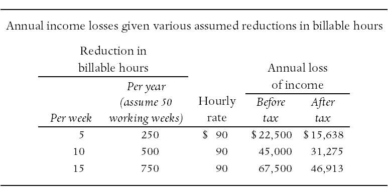
A case in which a plaintiff bills her services hourly, has no employees, and expenses that are mostly fixed (not increasing with additional billable hours), is almost an ideal scenario for estimating the loss. Her loss of income is directly linked to her ability to bill hours. Other cases can be much more complicated.

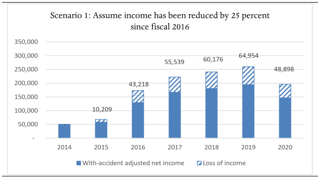
Another case that I worked on involved a plaintiff who was in the early stages of establishing his business when he was injured. Following the accident he was able to continue to grow his business, and his income increased accordingly. His business income was fairly complicated, with employees who also generated revenue, as well as numerous expenses. After estimating the income that he earned from his business, the potential loss of income was not at all obvious because his income had increased so much after the injury, as shown below.

Because the plaintiff was injured while he was in the early stages of establishing his business, I didn’t have a useful pre-accident history as a comparison. However, his business income was heavily linked to his ability to spend time at work, and to be productive during that time. Because of his injuries, it was claimed that he needed more many breaks at work and he was not able to perform some of the more lucrative jobs that would normally have been available to him. Effectively, the evidence was suggesting that if he was uninjured, his revenue and earnings would be much greater. The question of course, is how much greater? Ultimately I provided a range of scenarios, and one was that I assumed that his income has been reduced by 25 percent because of his residual deficits. (That is, he has only been earning 75 percent as much as he would have been earning if uninjured.) This is depicted in the chart below.

Clearly this is not as exact as we might hope, but providing a range of scenarios using this approach can at least provide an estimate of the loss if the Court accepts a certain set of assumptions. Dealing with a self-employed plaintiff can involve much more uncertainty than when we have (say) a teacher who is working three-quarters of full-time because of her injuries, rather than full-time.

Another approach that can potentially be useful is the replacement cost approach. In some cases it is possible for the plaintiff to hire a helper that will enable the business to continue as it would have in the absence of the accident, though with additional expenses (and reduced profit) due to the cost of the replacement worker. For example, an injured owner of a landscaping business might be able to hire a part-time labourer to assist him with some of the heavier tasks. If this helper is paid $40,000 per year, then business expenses will increase by $40,000 and profit will decrease by $40,000. That’s $40,000 that is not available to be paid to the owner, so his annual loss of income due to hiring the replacement worker would be $40,000 (not accounting for tax). In this case I am assuming that the self-employed landscaper can continue with the managerial aspects of his business, and he can perform some of the manual labour, but his residual deficits are preventing him from performing the heavier tasks.

The possibility of hiring a replacement worker is something that should especially be considered when the plaintiff is claiming that his income loss is particularly high. If the self-employed landscaper in my example above is claiming a huge annual loss, it is reasonable to ask why his loss is not capped at around the cost of a full-time labourer. But in other cases, the cost of hiring an assistant is not going to be a reasonable approach. For example, a surgeon with a back injury presumably cannot mitigate her losses by hiring a helper – her best option might be to take longer breaks in between procedures.

*   *   *

For a PDF version of this presentation, click here.

ACTLA Presentation – Without- and With-accident income: Total Compensation

ACTLA Lunch & Learn

Without- and With-accident income: Total Compensation

Prepared by:

Kelly A. Rathje, MA

Without- and With-accident Income: Total Compensation

In the sections below, I provide notes that I used to discuss the different sources of earnings data experts can rely on to estimate an individual’s earning stream, and other sources, usually benefits, that make up an individual’s total compensation.

1 Sources of Earnings Data

When doing a loss of income calculation, we need to estimate both the without- and with-accident income streams. That is, we need to determine what the individual would have earned, had the accident not occurred, and what that individual will earn now, despite the injuries.

1.1 Average of past income

We can look at an average of the individual’s past income, both before and after the accident. If they have a well-established income stream prior to the accident, then assuming that they would have continued to earn the same level of income that had been achieved prior to the accident is usually a reasonable representation of what they will earn in the future. Similarly, if they have an established income stream after the accident, it is a good indicator of what they are capable of earning, despite their injuries.

However, there is a downside to relying on a average of past income, as it  may not account for future promotional wage growth. Also, it may reflect earnings during a boom time in the economy or a slower time (recession) during the economy. For example, if in the oil industry, relying on earnings during the 2010-2015 time frame, although we have 6 years, it may overstate the without-accident earnings since this was during a boom in the oil industry. Similarly, relying on average earnings for the 2015-2020 time frame may understate due to the significant decline in the oil industry.

1.2 Census data

Another source of earnings data is the Canadian Census. This source is the single most reliable source of earnings data in Canada. It provides earnings data for specific occupations, age categories, gender, and education.

Census data if very useful when an individual has just completed their education and are started a career; or only has been working for a few years in an occupation; or has changed occupations during their work. It is also useful when an individual does not have a well-established career (income) path, as in the case with younger individuals. In the with-accident scenarios, it is often the case that the injured party needs to retrain, so to estimate the earnings stream we can look at census data for individuals within the same occupation, and the same level of education.

The census data can also provide a baseline comparison when considering an individual’s average of their past income. It can help us determine if the individual’s earnings are consistent with what statistical averages would suggest, or if they are above- or below-average.

1.3 Salary grids/Collective bargaining agreements

Certain occupations have their salaries and/or wage rates specified by a collective agreement. Two examples of such occupations are teachers and nurses.

The collective agreements and salary grids are a useful source of earnings data as it exactly sets out how an individual’s earnings will progress. For example, the teacher’s salaries are specified for the first year of teaching through the tenth year of teaching – at which time they reach the top of the salary grid. Since teachers do not tend to receive overtime pay or shift differentials, if the school division the individual is going to work for is known, then we know exactly how the salary will progress with experience.

Another example of an occupation with a salary grid is nursing. As you gain experience, the wage rate increases such that after nine years of experience, the top of the salary grid is reached. However, with jobs like nursing, the salary grid reflects the base wage rate. A nurse’s wage if often higher than the base rate due to things like overtime, shift premiums, and education premiums. However, the base wage rate is still useful when estimating the income of a nurse.

First, if the individual has an established income stream as a nurse, the base wage rate, and the reported employment income, can be used to determine “straight-time equivalent hours” (STE). The STE hours are the number of hours a person would have to work, at their base hourly wage, in order to earn the same income they earned after receiving shift premiums, overtime hours, education premiums, lump-sum pay-outs, and so forth. The STE hours, and the base wage rate can then be used to estimate a future income stream.

Second, if there is not an established career, the base wage rates can be used to estimate a wage inflation index, and this index, specific to the nursing occupation, can be applied against the census data (which is reported in 2015 dollars), to determine an income stream, in combination with the census data.

2 Other sources that make up total compensation

In addition to money paid to an employee, an individual may also receive benefits as part of their total compensation for employment. These sources should also be taken into consideration when calculating the income streams for a loss of income assessment. These are usually included under the heading “fringe benefits”.

2.1 Insurance

Extended health, disability, dental, life. This is a benefits package that an employer provides to an employee, and is usually valued at approximately 2.5 to 3.5 percent of earnings, and we usually include the value of insurance as a percentage of income.

2.2 Car allowance

The employer may provide compensation for vehicle use, or provide a company car. This is usually a taxable benefit, and the value of the benefit is already included in the reported T4 earnings (box 34 of the T4 slip).

2.3 RRSP matching

This benefit arises when the employer makes contributions to an RRSP, matching the employee’s contribution to a certain percentage. This is also usually a taxable benefit, and already included in the reported T4 earnings (box 40 of the T4 slip).

2.4 Stock/security options

 This benefit is offered as an offer to purchase shares of the company, at some specified price. The individual may then choose to sell these shares, once they’ve vested, in order to realize a profit on the sold shares. If this option has been exercised in the past, then the net value of the sale is usually a taxable benefit and already reported in the T4 earnings (box 38 on the T4 slip). In this particular case, the cost of the stock option needs to be deducted in order to determine the net value of the sale. The cost is reported in box 41 of the T4 slip. For example, suppose the option to purchase 10 shares is offered at $5 per share. Once it vests, it is sold at a market value of $10 per share. The $100 (= $10 × 10 shares) would be reported as T4 earnings, but the cost of the option $50 (= $5 × 10 shares), which is reported in box 41, would need to be deducted.

There are also cases in which the stock options have no value. For example, suppose the option to purchase 10 shares is offered at $5 per share. Once it vests, the market value of the share is only $2.50 per share. In this case, the cost to purchase the option ($50) is more than what would be received for selling it ($25), so the option has no value.

Stock options do not seem to be that common, and when estimating the value of potential future stock options, we usually include the value of a percentage of income.

2.5 Employer-funded pensions

There are two types of employer-funded pensions. A defined-contribution and define-benefit.

Defined contribution

A defined contribution plan is simply whatever is contributed on the individual’s behalf is what is received out. If the employer contributes 10 percent of earnings, then the value of the employer-funded pension benefit in each year is 10 percent. This is included as a percentage of income.

Defined benefit

A defined benefit pension plan is when both the employer and employee make contributions to the plan, and upon retirement, a formula is used to calculate the pension benefit. Examples of a defined benefit pension plan are the Local Authorities Pension Plan (LAPP), the Alberta Teacher’s Retirement Fund (ATRF), police forces, and so forth.

The value of the defined benefit pension plan can be captured in two ways. First, the value of the employer’s contribution can be included as a percentage of income. Thus, the employee will receive the employer contribution as part of their loss of income. The amount that the employer would have contributed on their behalf can be invested in a private pension plan. Upon retirement, the reduced with-accident pension plus the top-up from the private plan investment, will equal the without-accident pension, thus ending the loss.

A second method to capture the value of the employer-funded pension is to actually calculate the without- and with-accident pension streams upon retirement, and compare the two to determine the loss of income.

2.6 CPP pension

It is assumed that the premiums an employee pays into the Canada Pension Plan (CPP), are roughly equivalent to what that individual will receive as a retirement pension. It seems logical that if an individual is earning less than they would have, had they not been injured, they will not be contributing as much to the pension plan. As a result, the with-accident retirement benefit will be less than in the without-accident scenario. This may not be the case.

For example, if the individual is receiving CPP disability, and will continue to receive disability until age 65, the CPP retirement benefit may not be impacted as all of the years on disability are ignored when calculating the benefit.

Second, if the individual would have earned, and will earn, an income at least as much as the yearly maximum pensionable earnings, then the contributions (and resulting retirement pension) will be the same in both the without- and with-accident scenario.

However, if there is a difference between the without- and with-accident CPP contributions, then it is reasonable to include a percentage of income to reflect the difference in premiums. As an example, suppose in the without-accident scenario, an individual would have earned $100,000, and after being injured, they earn $45,000. The CPP contribution in the without-accident scenario would be $3,166 (the maximum) but in the with-accident scenario would be $2,262. This is a difference of approximately $921 per year. In this particular case, it could be reasonable to include a 3 percent contingency in the without-accident scenario and a 5 percent contingency in the with-accident scenario to reflect the difference.

For a PDF version of this presentation, click here.

Are Data from the 2011 Census Reliable?

by Christopher J. Bruce

When estimating future earnings in personal injury and fatal accident cases, financial experts often rely on information provided by the Canadian Census. Of particular importance are data concerning incomes by age, sex, occupation, and education. For example, if a 24 year-old male plaintiff would have been a journeyman carpenter, his potential earnings might be based on average incomes for Canadians with that certification, in the age groups 25-29, 30-34, 35-44, etc.

In the past, these data would have been drawn from a section of the Census known as the “long form.” This portion of the Census survey, which contained much more detailed information than on was on the rest of the Census, was given to only one household out of five. (The remainder of the Census survey asks only basic questions about such demographic factors as age, sex, language, and area of residence.)

For the 2011 Census, however, the government decided to replace the long-form questions with a “National Household Survey (NHS).” Although the 2011 NHS asked the same questions as had the 2006 Census long form, whereas the long form had been mandatory, the NHS was voluntary. The result, as had been expected, was that the percentage of households answering this portion of the survey fell significantly, from 93.8% in 2006 to 77.2% in 2011.This created three statistical problems concerning the reliability of the data (variability in small community data, sample error, and non-response bias). As Statistics Canada had anticipated these problems, however, it took steps to mitigate them, steps that have maintained the reliability of the data that are of value to the courts. Wayne R. Smith, Chief Statistician of Canada, recently wrote an article in which he discussed these steps. [“The 2011 National Household Survey – the complete statistical story,” http://www.statcan.gc.ca/eng/blog-blogue/cs-sc/2011NHSstory. June 4, 2015.] In this article, I summarise Dr. Smith’s discussion.

Variability in small community data

As the sample size of any survey becomes smaller, the data become less and less reliable, due to an increase in variance. In response, Statistics Canada routinely withholds data concerning the smallest communities. In 2011, they withheld the results from 1,100 such communities, up from 160 in the 2006 Census. That is, all of the data reported in 2011 meet the normal statistical requirements for reliability.

Sample error

As the overall size of a sample decreases, there is an increase in what is known as the “sampling error;” that is, from the problem that the average characteristics of the sample differ from the average of the total population. Because Statistics Canada expected a smaller percentage of households to answer the voluntary NHS than had answered the mandatory long form, they anticipated that the total size of the “sample” (the households answering the survey) would be lower in 2011 than in 2006.

To deal with this problem, Statistics Canada increased the number of households who were asked to answer the long portion of the 2011 Census. Whereas one household in five were asked to answer the 2006 long form, one household in three were asked to answer the NHS. The result was that, even though a smaller percentage of households responded to the NHS than had responded to the 2006 long form, the number of households answering the NHS was higher than in 2006, (2,657,461 versus 2,443,507, representing 6,719,688 versus 2006’s 6,136,517).

Although this approach does not correct for all errors, those errors become less and less important as the data are aggregated. Thus, for example, the data for the average income of all carpenters in Alberta are more reliable than for the average income of carpenters in Calgary.

Non-response bias

The most worrisome problem that arises when a survey is made voluntary is that the households who choose to respond to that survey may differ significantly from those who refuse to do so. For example, if those carpenters with relatively high incomes are more likely to respond to the NHS than are those with low incomes, the average incomes reported by the NHS will be biased upwards.

Statistics Canada could not control, ex ante, for the possibility that this would happen. However, they were able, ex post, to investigate whether the respondents to the NHS were representative of the overall groups from which they were drawn – that is, they were able to determine whether the respondents “looked” different from the average.

To make this determination, Statistics Canada was assisted by the fact that they had a considerable amount of information about the respondents to the NHS before those individuals answered the NHS survey. Most importantly, they also had their responses to the short questions on the Census that are mandatory for all Canadians. In addition, they were also able to link the NHS respondents to those individuals’ tax files, immigrant landing data, and the Indian Register.

Using sophisticated statistical techniques they were able to determine that the average respondent to the NHS had very similar characteristics to the average Canadian with respect to age, sex, language, area of residence, income tax, immigration status, and aboriginal status. This finding leads Statistics Canada to conclude that the NHS respondents were, in most cases, representative of the larger population from which they were drawn. And when Statistics Canada was unable to conclude that the individuals who replied to a specific sub-class of questions were representative of the population, the resulting data were not released, or they were released with an accompanying cautionary note.

Summary

To summarise: Although the long-form portion of the 2011 Census was made voluntary, there is sound reason to believe that the data that are of greatest relevance to the calculation of lost earnings can be relied upon.

  1. The information in this article is drawn from a blog written by Wayne R. Smith, Chief Statistician of Canada, entitled “The 2011 National Household Survey – the complete statistical story,” June 4, 2015. This blog can be found at: http://www.statcan.gc.ca/eng/blog-blogue/cs-sc/2011NHSstory.


Christopher Bruce is the President of Economica and a Professor of Economics at the University of Calgary. He is also the author of Assessment of Personal Injury Damages (Butterworths, 2004).

The Impact of Childhood Sexual Abuse on the Educational Attainment and Adult Earnings of Canadian Women

The Impact of Childhood Sexual Abuse on the by Christopher J. Bruce, Ph.D. & Daniel V. Gordon, Ph.D.

This article first appeared in the autumn 2007 issue of the Expert Witness.

Introduction

One of the most complex issues facing the courts in any sexual abuse case is the determination of the impact that the harm has had on the plaintiff’s earning capacity. Not only is very little statistical evidence available on this issue, but the data that do exist have often proved to be unreliable.

Recently, this lack of a reputable source has been resolved with the publication of a Statistics Canada survey in which a representative sample of Canadians was asked about their experiences of victimization. From this survey, we were able to obtain information about a large set of (adult) women who had suffered sexual abuse as children.

The purpose of this paper is to report our findings concerning the consequences of that abuse on the educational attainment and earnings of the victims. Our surprising result is that, among most such victims, abuse does not have a statistically significant effect on adult education and earnings. Furthermore, in the only group for which abuse
was found to have a significant effect – women who were first abused between the ages of seven and thirteen
– education and income were higher than among women who had not been abused.

The remainder of the paper is divided into three sections: a review of the existing literature; the development of an economic model concerning the effect of abuse; and a summary of our statistical findings.

Existing Literature

The academic literature concerning the effects of childhood sexual abuse is composed of two streams. In the first, researchers have attempted to develop theories of childhood social-psychological development that can be used to understand the pathways by which abuse affects its victims. In the second, researchers have used statistical tests to identify correlations between abuse and its predicted outcomes, such as depression, alcoholism, and school completion rates.

Theoretical

Many theories concerning the impact of sexual abuse are founded on the ‘core-symptom’ model, in which a
core problem or event is presumed to have led to one or more symptoms. The most common of these models characterize sexual abuse as a trauma, leading researchers to predict that abuse will result in post traumatic stress disorder.

An alternative interpretation suggests that, rather than
having a single effect, sexual abuse might produce multifaceted effects. Finkelhor and Browne (1985), for example, argued that sexual abuse had four primary effects: traumatic sexualization, stigmatization (i.e. low esteem and self-destructive behaviour), betrayal, and powerlessness.

A third approach, ‘developmental models,’ proposes that sexual abuse may affect victims by interfering with development in areas such as social- and self-functioning. In this view, therefore, the age at which the child is abused may be a critical determinant of the long-term effects of that abuse. For example, Celano (1992) suggested that the impact of sexual abuse may differ among Piaget’s three stages of childhood moral development (Piaget, 1965): preschool (ages 0-6), latency (7-13), and adolescence (14-19). She hypothesised that whereas preschoolers may not recognise that abuse is morally reprehensible, and adolescents may consider their moral culpability to be ameliorated by failure to provide informed consent, children in the latency period may consider themselves (at least in part) to be responsible for many of the types of abuse. Accordingly, she predicts that abuse will be most harmful if it occurs in the latency period.

Statistical

Statistical studies can roughly be divided among those that investigate the effect of sexual abuse on: psychological factors, (such as depression, self-esteem, and sexuality); social outcomes, (such as alcoholism and delinquency); and economic outcomes, (specifically, schooling and adult income).

This literature is virtually unanimous in its finding that childhood sexual abuse has statistically significant effects on the victim’s psychological well-being. The outcomes that are most commonly found include: low self-esteem, post-traumatic stress disorder, depression, affective and personality disorders, and anti-social behaviour.

The sociological literature has provided evidence concerning the effect that abuse has on criminal activity. Studies that aggregate across a number of different types of childhood abuse
– neglect, physical abuse, and sexual abuse, for example
– commonly find that criminal activity is correlated with
this aggregate; although some find no statistically significant correlation. Importantly, however, when ‘abuse’ is separated into its components, it is only ‘neglect’ that is found to be correlated with criminal activity. Neither physical nor sexual abuse appears to be a significant determinant in this formulation.

Very mixed results have been obtained when researchers investigate the impact of abuse on schooling and income. Slade and Wissow, (2006) found that individuals who had been maltreated as children had lower high school GPAs than the control group, but no greater problems with teachers, with completion of homework, or with school absences. And some studies have found evidence that victims of childhood sexual abuse performed better in school than those who had not been abused (e.g. Eckenrode, et al. 1993 and Buckle, et al. 2005).

Economic Model

In our model, we assume that individuals divide their time among three activities: solitary leisure activities, such as reading, watching television, and playing video games; social leisure activities, such as team sports, club memberships, and interacting with friends; and “market” activities, such as investing in education and working in the labour market. The value of each activity increases as additional time and effort is devoted to it. And the “cost” of time spent in any one activity is the value that is foregone from the other activities (the “opportunity cost” concept so familiar to economics students).

We hypothesize that the effect of sexual abuse is to reduce the benefits that individuals obtain from each of the three activities. Normally, one would expect that this would lead to a reduction in each of them. However, assume that the negative effect on the time and effort devoted to two of the activities was greater than it was on the remaining one. In that case, it is possible that the victim might “substitute” away from the more seriously-affected activities towards the less-seriously affected one. As a result, the latter might even increase.

For example, if abuse had a much more significant (negative) impact on the individual’s ability to socialize than on
her ability to undertake schoolwork or to compete in the labour market, abuse might lead to a lesser reduction in the latter activities than expected, and could even lead to an increase in those activities. In common parlance, the individual might be said to have compensated for the harm to her socialization skills by ‘throwing herself’ into academic and work-related activities. In such a case, abused individuals might be observed to complete more years of education than the non-abused, and might earn higher incomes; but this would come at the expense of a significant withdrawal from normal social activities. We propose to test for this effect in the analysis reported in the next section.

Statistical Estimates

We obtained information concerning 6,528 adult Canadian
women, (drawn from the 1999 General Social Survey), of whom 607 reported that they had been sexually abused as children. Using the data from this survey, we conducted two statistical tests.

In the first of these, we estimated the effect of a series
of variables on educational achievement. The variables that are usually found to be important – such as parents’ education, individual’s place of birth, and whether the individual belonged to a “visible minority” – all proved
to be significant in our data. In addition, we found that if the individual had first been sexually abused between the ages of seven and thirteen, she obtained more education than did individuals who had not been abused or who had first been abused before seven or after thirteen.

In our second test, we estimated the effect of a number of background variables on adult earnings. As expected, we found that variables such as the individual’s education and whether she belonged to a visible minority had significant effects on income. And, again, we found that individuals who had been abused between the ages of seven and thirteen had statistically higher levels of income than did those who had not been abused or who had first been abused before seven or after thirteen. Importantly, this effect is in addition to the increase in income that would have arisen from the effect of abuse on education.

To summarise, we found: first, that abuse before the age of seven or after the age of thirteen had no statistically discernable effect on either the victim’s education or her adult income. Second, abuse between the ages of seven and thirteen increased average educational levels and increased average incomes, both directly and indirectly (through the effect on education).

Conclusion

We have found that, on average, sexual abuse is not associated with lower educational levels or lower adult incomes among victims. This does not mean that all victims have higher income levels than those who have not been victimised: some victims will be above-average and some below. When the court is dealing with a particular plaintiff, it should always rely on factors that are specific to that individual. Nevertheless, our results suggest that it cannot be concluded, without such specific information, that the individual’s adult income will be adversely affected by sexual abuse.

References

Buckle, S., S. Lancaster, M. Powell, and D. Higgins (2005) “The Relationship Between Child Sexual Abuse and Academic Achievement in a Sample of Adolescent Psychiatric Inpatients,” 29 Child Abuse and Neglect, 1031-1047.

Celano, M. (1992) “A Developmental Model of Victims’ Internal Attributions of Responsibility for Sexual Abuse,” 7 Journal of Interpersonal Violence, 57-69.

Eckenrode, J., M. Laird, and J. Doris (1993) “School Performance and Disciplinary Problems Among Abused and Neglected Children,” 29 Developmental Psychology,
53-62.

Finkelhor, D., and A. Browne (1985) “The Traumatic Impact of Child Sexual Abuse: A Conceptualization,” 55 American Journal of Orthopsychiatry, 530-541.

Piaget, J. (1965) The Moral Judgement of the Child, (New York: Free Press).

Slade, E., and L. Wissow (2006) “The Influence of Childhood Maltreatment on Adolescents’ Academic Performance,”
Economics of Education Review, (in press).

leaf

Christopher Bruce is the President of Economica and a Professor of Economics at the University of Calgary. He is also the author of Assessment of Personal Injury Damages (Butterworths, 2004).

Daniel V. Gordon, Ph.D., is a professor of economics at the University of Calgary, where he specialises in the use of statistics for economic analysis.

Increased Earnings After Injury

by Michael Behr

This article was originally published in the autumn 1999 issue of the Expert Witness.

Has an injured person sustained a loss if the injury forces a change in occupation which produces higher income? Definitely. Any suggestion that injury is beneficial contradicts fundamental economic principles.

Resources

Economics allocates resources to competing uses which forces choice. The possession of a higher quantity and quality of resources is the power to realize more valuable choices. Injury, virtually by definition, is a reduction in the quantity or quality of resources possessed by the injured party. Therefore, injury constitutes economic loss.

Cross Section versus Time Series

Sleight of intellect puts damages into time series and concludes that higher post-injury income shows no loss. But the issue in damages is not the time series difference between yesterday without injury versus today with injury. Rather, damages are the cross sectional difference between today without injury and today with injury. Time series violates the required ceteris paribus conditions because the passage of time incorporates many changes in addition to the injury itself, most notably of course, the occupational change producing the higher income.

The naïve are seduced by the replacement of cross section with time series because life is lived in time series, whereas the cross section requires abstraction from experience to comprehend the alternative condition after injury but without the injury. The skilled tortfeasor defendant can be expected to attempt to substitute time series for the cross section if it leads to a lower or negative loss conclusion because of higher post-injury income. That defendant is emboldened by the realization that time series will probably have intuitive appeal to a jury. Plaintiff must therefore be vigilant and unyielding in preserving the cross section. If not, the defendant making an invalid argument to an economically naïve jury has an excellent chance of producing a perverse verdict to the detriment of plaintiff. Perverse verdicts are inconsistent with market values and therefore also reduce the general welfare of society.

Information

The thoughtful may attempt to rebut the above, arguing that information is central to the allocation of resources to their most valuable ends, citing the role of information as a condition of a competitive economic system. Inasmuch as it was the injury that “informed” plaintiff of the higher income opportunity, it is argued the damages should be credited with the higher income itself. This argument contradicts fundamentals underlying a market economic system in a society valuing individual liberty.

Noneconomic Values

The higher income opportunity undoubtedly existed prior to
the injury, but may have been rejected for noneconomic reasons. The disutility of the higher income employment may exceed the value of the higher income itself in the eyes of plaintiff. If so, forcing plaintiff to credit the damage with the higher income is to force plaintiff to substitute uncompensated noneconomic loss for what would otherwise be compensated economic loss.

Antisocial Incentives

Accepting the argument for crediting the damage with the higher income leads to the conclusion that I should waken my sleepy neighbor by disabling him to force him to replace his physical occupation with more sedentary higher employment. Further, he should pay me for this valuable service. This absurdity is a direct incentive to destroy resources, which in a world of resources insufficient to satisfy all competing ends is inimical to the interests of society.

Collateral Source

The economic essence of collateral source is compensation for injury occasioned by the injury itself. Generally, defendant is barred from a credit against liability for damage from collateral sources on the grounds that the social interest is served by not allowing a tortfeasor to escape the cost of his acts. This position is consistent with market economics where parties bear the cost of their actions in exchange for reaping the benefits. Although the discovery of a higher income occupation occasioned by an injury is not included as a collateral source in the law, its economic character is that of collateral source. The tortfeasor may not benefit from it as a matter of economics-and ideally in the law as well for whatever reason.

Mitigation

At some point collateral source comes into tension with the economically valid legal requirement that plaintiff must make the best of it under the circumstances. The market expects resources to find their way to their highest and best uses, including those held by injured plaintiff. This works to the benefit of tortfeasor and may include some obligation by plaintiff to move to a more suitable post-injury occupation which may turn out to be higher paying. How much disruption of plaintiff’s life to accommodate his/her injury is a reasonable obligation of plaintiff? Is he/she required to move to another planet, so to speak, to realize the higher income?

The consequence of this tension is that the damage will be bounded by the cross sectional differences between pre-and post-injury income in the pre and post-injury occupations. Inasmuch as the adequacy of plaintiff’s mitigation is inevitably directly or indirectly a jury question, the economist may be well advised to provide a damage conclusion based on the effect of the injury on both the pre-injury earning capacity in cross section and on the higher post-injury earning capacity in cross section. The injury’s hindrance of performance in the higher income employment may actually be greater than its hindrance of the pre-injury occupation in cross section. An expert vocational opinion may be a foundational requirement for each occupation.

If there are retraining or other costs to plaintiff necessary to realize the higher post-injury income, the value of the higher income must, of course, be net of those costs.

Conclusion: The destructiveness of an injury establishes the fact of an economic loss irrespective of pre and post-injury incomes or earning capacity. Plaintiff’s competitive position, and therefore his range of choice in the market is reduced by the injury, legal prohibitions of discrimination against the disabled notwithstanding. The forensic economist’s damage conclusion is, at its core, the value of that reduced range of choice.

leaf

Michael Behr is a forensic economist located in Northfield, Minnesota. He holds a Ph.D. in Agricultural Economics from the University of Wisconsin-Madison. From 1969 to 1983 he was Associate Professor and Professor of Business and Economics at the University of Wisconsin-Superior teaching most undergraduate economics courses and statistics. Tired of University meetings, memos and the same old track by 1983, he resigned his University position for the greater fun and profit of full-time self-employment as a forensic economics sole practitioner. He has been involved in about 1,300 cases, about half of them small business matters with the majority of those farms and other agricultural matters. He may be reached at P. O. Box 430, 813 N. Linden St., Northfield, MN 55057. Phone 507-663-7124. Fax 507-663-1735. mbehr@mrb.com.

Injured, Yet Better Off?

by Scott Beesley

This article was originally published in the summer 1999 issue of the Expert Witness.

We occasionally encounter the claim that a plaintiff is better off financially than before the accident, or at least will be better off in the future. The evidence for this is usually that they are now earning more than they did at the time of the accident. Therefore how can there be any loss? This is not really very hard to respond to, and there are several reasons why there may still be a modest, or very substantial, loss of future income.

In an article in the March 1999 Barrister, Mr. Cameron J. Ashmore of Russell & Company provided a discussion of this issue, within a broader analysis of possible approaches to future loss assessment. Mr. Ashmore listed four reasons why a person who was apparently earning more might still have a loss of future income: early retirement, increased risk of unemployment, reduced future wage growth, and the prospect of time missed from work over the years. All of these are certainly legitimate concerns, and we commonly address them in our work. They all require, however, subjective judgments regarding the future effects of injury, which are difficult even for vocational experts to assess. If vocational opinions are not provided, or if the plaintiff’s outlook is less than clear, then we commonly consider a range of alternatives
(i.e. various growth, contingency and retirement assumptions). The court can then choose the figures it finds most reasonable in the pre- and post-accident cases, and the loss follows from that. If the court, for example, finds that all of these effects are fairly minimal, then indeed a small future loss is all that will result.

There is another issue to consider in these cases, and that
is wage growth between the date of the accident and the date of the evaluation. I would suggest that in some cases, a future loss is denied on the basis of faulty logic, in that
post-accident wage growth in that period is accepted as a fact, while pre-accident wage growth is implicitly or explicitly not considered. We refer now to wage growth in the general sense of any career progression, either incremental or sudden (such as when improved educational standing leads to a quick increase in income). It should be quite obvious that, no matter how minimal the injury, a plaintiff is never more capable of vocational progress after an injury than before, yet that is commonly implied or suggested outright.

Consider the example of an average male college graduate, injured at the age of 27, when he was earning $32,000. Five years later, at age 32, he is earning $33,000. First, we note that inflation alone applied to the older figure would probably predict an income of roughly $34,500, so even with just that adjustment there is an immediate loss. Much more important is the fact that 1996 Census data would predict that over those 5 years, the plaintiff’s income would have grown by approximately 22.56 percent, plus inflation. Assuming cumulative inflation of 8 percent over the five years, the total estimated increase in pre-accident income is 32.36 percent, and the value of pre-accident income at age 32 is
$42,355. The loss from age 32 to 33 is seen to be approximately
$9,355, and of course this loss may continue through to retirement. (In many cases the annual loss will decrease over time, simply because an average income curve starts with higher growth and levels off, such that a plaintiff who is five years behind, for example, will eventually get closer to their pre-accident level.)

I realize that the above example seems quite trivial, but we have repeatedly seen analyses in which post-accident figures are compared to pre-accident income from several years before, and inflation, or pre-accident wage growth, or both, are ignored. While there is certainly room for argument regarding how much more pre-accident wage growth a plaintiff might have enjoyed, it can never be considered logical to say that they will enjoy better prospects and wage growth after being injured. It is also flatly wrong to compare a post-accident figure to a pre-accident figure from several years before, without adjusting for inflation.

When a high school graduate plaintiff, in another example, retrains 4 years after the accident, and obtains a diploma in technology, their income could easily be far greater than before the accident. I would suggest that it is generally wrong to suggest that there is no future loss. I would further suggest that one fair way to assess the loss is to assume that the plaintiff would have completed the same given diploma one to three years sooner, in the absence of the accident. The loss then is the gap between pre- and post-accident income curves, which, as noted above, could almost vanish when growth slows in the later years of the person’s career. If the plaintiff had had no plans to enter such training until the accident occurred, that should not prevent the use of the method: clearly he/she had the potential to enter some form of training, and any such upgrade would have resulted in increased income. In addition to the loss resulting from a lag of some years, it is also possible that some of the four factors Mr. Ashmore listed will also be found to apply, and a more substantial loss might result.

In the absence of evidence regarding the plaintiff’s intentions prior to the accident, it is reasonable, I would argue, to assume that the plaintiff would have followed the same career path had the accident not occured as he/she has been observed to follow after the accident. If the new field is about as lucrative as any they could have entered, without injury, then there is probably no loss beyond what is due to the time lag and, possibly, some increased contingency risk. The loss is limited to the delay and probably some increased contingency risk. Conversely, the defense should not be able to claim that, because of the accident, the plaintiff has entered a new and better-paying field. To do so is, I repeat, to deny that the given path was possible before the injury, which makes little sense.

Two other examples merit brief mention. The first concerns women who are becoming more involved in work, after their children reach some particular stage (e.g. into grade 1). In such cases we might see a woman who had had very minimal income enjoy significant increases, even after an accident. This is occurring because they can now use their earlier training, or commit to full-time work, or move, or simply devote time to retraining and adding to their employability. It is again false to compare the income such a woman is now earning to what they were earning perhaps 6 years ago, yet this has been done at times. Any correct pre-accident scenario must be an answer to the question “What career path would have been open to Ms. Plaintiff, in the absence of the accident, and considering that her children are older and she can devote more time and energy to work?” One cannot use a pre-accident income level from the past, as if, in the absence of the accident, the children would never have grown up!

A final example is similar in principle to the case of the
“returning mother.” I have handled a fatal case in which pre-accident business income was assessed using the average of several years prior to the accident. As it happened, these were very poor years for the type of business in question, with returns well below the historical average. At about the same time as the accident, the business climate improved dramatically, producing higher returns for the surviving spouse, who was using a family member to replace some of the deceased’s labour. The opposing expert used income from the poor, before accident years to estimate pre-accident income, and an average in the later good years to define post-accident income. The plaintiff was said to be better off, before accounting for the (inadequate) wage paid to the family member to replace the deceased’s labour. After that was subtracted, the plaintiff was said to have suffered only a very slight loss. Note that this entire treatment is fatally flawed, as it assumes that the deceased would never have benefited from the improved business climate. Alternatively, it amounts to claiming that the accident
caused that improved business climate, which seems even more indefensible.

Any loss assessment should properly address the financial effects of changes which are due to the accident, and those alone. Other unrelated changes must be applied in both the pre- and post-accident analyses. Failure to compare apples to apples is an objective wrong, not simply a point of legitimate subjective dispute, like many of the assumptions made in most loss of income reports.

leaf

Scott Beesley is a consultant with Economica and has a Master of Arts degree (in economics) from the University of British Columbia.

Distinguishing Between Loss of Income and Loss of Earning Capacity: The B.C. Case of Pallos v. I.C.B.C.

by Scott Beesley

This article first appeared in the summer 1996 issue of the Expert Witness.

In its recent decision in Pallos v. Insurance Corporation of British Columbia (1995, B.C.J. No. 2), the British Columbia Court of Appeal awarded $40,000 for “loss of earning capacity” to a plaintiff who had no “loss of earnings.” The basis of the claim was that, although the plaintiff had returned to his previous employment, at a salary commensurate with that earned prior to the accident, the injury had diminished his future job prospects.

Pallos raises an important issue which is often given less attention than it deserves in personal injury actions: how should the court deal with uncertainty concerning the course of the plaintiff’s future earnings stream? In Pallos the uncertainty was of an extreme form, as it was unclear whether the plaintiff would have sought alternative employment had he not been injured nor was it certain what effect the injury would have on the post-accident probability that he would be able to keep his job or to find another one.

Other cases present the courts with varying degrees of uncertainty. In this article, I consider four types of uncertainty, in increasing order of complexity. The fourth case represents the situation which was dealt with in Pallos.

At the lowest level of complexity, the court has determined what career path the plaintiff will follow (or would have followed) but is uncertain concerning factors specific to that career, such as the rate of growth of earnings, the level of fringe benefits to be paid, the probability of unemployment, or the age of retirement. This common form of uncertainty can be, and is usually, dealt with simply by using averages. Although different automobile mechanics may experience different rates of growth of earnings, for example, it is generally appropriate to assume that the plaintiff’s income would have experienced the average rate of growth of earnings, for mechanics with characteristics similar to those of the plaintiff (such as education, specialisation, and work experience).

At the second level of complexity, there is a dispute concerning the plaintiff’s career choice. Commonly, for example, the defendant will argue that an injured automobile mechanic should return to his previous employment (perhaps at a reduced capacity), whereas the plaintiff will argue that the plaintiff should retrain as a partsman. Often, this type of dispute can be resolved on the basis of an appeal to the facts. That is, it is often open to the court to argue that the facts indicate that one of the two (or more) courses of action is much more reasonable than the other. (The court might find, for example, that the plaintiff’s back injury is so severe that it is highly unlikely that he could resume his career as a mechanic.)

In the third situation, there are (or were) two or more careers open to the plaintiff, each of which is (or would have been) plausible. For example, it may be unclear whether the plaintiff would have taken a drafting diploma at a technical school or an engineering degree at university had she not been injured. The present, or lump-sum, value of the former would have been $700,000, whereas that of the latter would have been $1,100,000.

The court could employ the second approach identified above, and make a finding of fact concerning which of these streams the plaintiff would have followed. But the better course, I would suggest, is to weight each possibility by the probability that it would have occurred. This provides what is commonly referred to as a “weighted average” (or, technically, an “expected value”). For example, if it was felt that pre-accident there was a slightly higher probability that the plaintiff would have become a draftsperson than an engineer, the court might conclude that the probability of the former was 60 percent and that of the latter 40 percent. In this case, the weighted average of the two possible income streams would be:

Weighted average (pre)

= (0.60 x $700,000) + (0.40 x $1,100,000)
= $420,000 + $440,000
= $860,000

It is from this figure that the lump sum value of the post-accident income stream would be deducted in order to obtain the lump sum loss of future earnings.

The weighted average calculation, also referred to as the use of “simple probability,” has a long history of acceptance in Canadian courts. An early example is Bradenburg v. Ottawa Electric Railway (1909), 19 O.L.R. 34 at 36 (C.A.). Subsequent cases include MacDonell v. Maple Leaf Mills Ltd. (1972), 26 D.L.R. (3d) 106 at 109 (Alta. C.A.), Schrump v. Koot (1978), 18 O.R. (2d) 337 (C.A.) and Janiak v. Ippolito (1985), 16 D.L.R. (4th) 1 at 20 (S.C.C.). In the latter case the Supreme Court noted that “In assessing damages the court determines… what would have happened by estimating the chance of the relevant event occurring, which chance is then to be directly reflected in the amount of damages” (emphasis added).

Recent cases which apply this principle include Graham v. Rourke (1991), 74 D.L.R. (4th) 1 at 12-13 (Ont. C.A.) and Steenblok v. Funk (1990), 46 B.C.L.R. (2d) 133 (C.A.). Many other references, and a detailed discussion of related issues, can be found in Ken Cooper-Stephenson’s book Personal Injury Damages in Canada (2nd ed., Carswell, 1996), and I would like to acknowledge that the above citations were found in this text.

Use of the weighted average approach avoids a common problem in personal injury litigation – that the plaintiff may appear to be “better off” following the accident than before. For example, assume in the case above that the effect of the accident has been to increase the probability that the plaintiff will become a draftsperson from 60 percent to 80 percent – and decrease the probability that she will become an engineer from 40 percent to 20 percent. The defendant could argue that the plaintiff might have become a draftsperson before the accident and will now become an engineer after the accident, leaving her better off by ($1,100,000 – $700,000 =) $400,000.

The answer to this is that the defendant has ignored both the probability that the plaintiff would have become an engineer had the accident not occurred and the probability that she will become a draftsperson now that the accident has occurred. The best way to deal with this issue, we suggest, is for the court to weight each of the career opportunities by the probability that it would (will) occur and then to deduct the weighted average of the post-accident figures from that of the pre-accident. We already know in the case discussed above that the weighted average of the pre-accident earnings was $860,000. The comparable figure for the post-accident stream is:

Weighted average (post)

= (0.80 x $700,000) + (0.20 x $1,100,000)
= $560,000 + $220,000
= $780,000

Hence, the loss becomes ($860,000 – $780,000 =) $80,000. [Note: this calculation can readily be extended to cases in which there are three or four possible streams and to cases in which the numbers of streams pre- and post-accident are different.]

The final situation is that in which it is extremely difficult to attach probabilities to the possible future outcomes. This is the situation which was encountered in Pallos. There, the plaintiff had returned to his pre- accident employment, at an income which was similar to that which he had been earning prior to the accident. The court found that the nature of the plaintiff’s injuries was such that he would now have much greater difficulty obtaining employment with an alternative firm than he would have prior to the accident. What was unclear, however, were the probabilities that he would have sought alternative employment prior to the accident or that the firm would now lay him off, forcing him to seek alternative employment post- accident.

It might be possible to resolve this conundrum employing the weighted average approach; but the difficulties of obtaining appropriate probabilities make such a solution problematic. Implicitly, the two alternatives considered by the court were (i) to make no award; and (ii) to make a “fair assessment.” The B.C.C.A. chose the latter; Finch J.A. awarded $40,000 for what he called “loss of earning capacity.”

Although we sympathise with the approach taken by Mr. Justice Finch, we submit that it may be inferior to the weighted average approach. Given Mr. Pallos’ education and work experience, the number of opportunities realistically open to him had he left his current employer was limited. (Technically, the number may be unlimited, but most of his alternatives would have provided similar income levels.) Hence, the primary uncertainty to be resolved was the probability that he would have sought alternative employment. This is a probability which the courts in general could select, based upon the facts of the case. Similarly, the probability that a plaintiff like Mr. Pallos will be laid off from (or otherwise) leave his employer, post- accident, could also have been selected by the court. Although the selection of these probabilities may have to be based on subjective factors, I would suggest that the process of that selection would make the decision much more transparent and easier to translate to other cases.

This difficulty of translation has already become apparent. In Nelson v. Kanusa Construction et al. (1995, B.C.J. No. 958), a B.C. trial decision which followed Pallos, the plaintiff was awarded $50,000, also for “loss of earning capacity,” even though the award given to Ms. Nelson for loss of earnings appeared to have compensated her adequately.

Nevertheless, a substantial subset of cases may remain in which the plaintiff’s prospects are so uncertain that it is extremely difficult either to identify them all or to attach probabilities to them. In these cases, the Pallos approach – of providing a lump-sum to compensate the plaintiff for a loss of earning capacity – may be appropriate.

leaf

Scott Beesley is a consultant with Economica and has a Master of Arts degree (in economics) from the University of British Columbia.