Summer 2016 issue of the Expert Witness newsletter (volume 20, issue 2)

Contents:

This issue contains two articles. In the first, Christopher Bruce and Derek Aldridge examine the effect of a criminal record on earnings. In the second, Christopher Bruce and Kelly Rathje discuss the structure and content of expert cost of care reports.

The Effect of Incarceration on Future Earnings

  • In the first article, Dr. Bruce and Mr. Aldridge find that the literature regarding the effect of a criminal record on income suggests incarceration has a relatively small effect on lifetime earnings. Those who have been incarcerated tend to have lower levels of income than those without a criminal record, not because incarceration has changed their vocational/economic outcomes, but because they are drawn from a group with relatively low income to begin with. Further, the length of a person’s incarceration (holding the severity of the crime constant) appeared to have little impact on earnings, except in the case of “white collar” crime such as fraud or embezzlement. The literature suggests that individuals with supportive family ties, such as those living with their spouses and children, were the most successful at transitioning back into the workforce. In addition, the likelihood of recidivism decreased as an individual aged (i.e., those 30 and 40 year olds who were incarcerated in their early 20s are not likely to become repeat offenders).

The Structure of a Cost of Care Report

  • In the second article, Dr. Bruce and Ms. Rathje provide an economist’s perspective on various issues that arise in the presentation of cost of care reports. These include issues such as incremental costs, requirements that will vary over a plaintiff’s lifetime, the approach to ranges of estimates for costs or replacement frequencies, the costs of housekeepers and personal care attendants, and presentation. They also provide a sample calculation, to illustrate the issues discussed in the article.

The Structure of a Cost of Care Report

by Christopher J. Bruce, Kelly A. Rathje

As economists, we are often asked to calculate the present value of future costs of care. As these calculations are based on the reports of cost of care experts (CCEs), we have become uniquely familiar with the structure and content of those reports.

In this article, we provide a review of the format and contents of cost of care reports, drawn from our experience using those reports as inputs into our own calculations. We anticipate that this review will be of greatest use to:

  1. members of the bar: as a checklist against which to evaluate the cost of care reports that have been provided for them and their opponents;
  2. individuals who have recently begun preparing cost of care reports: to provide them with an understanding of how those reports will be used; and
  3. experienced cost of care experts: as an analysis of some of the complexities that can arise in personal injury actions. For these experts, most of our suggestions will be familiar; but we hope that we raise sufficient questions to make this report of interest to them also.

Incremental Costs

One of the most difficult questions facing the cost of care expert (CCE) is that of distinguishing between those costs that would have arisen had the plaintiff not been injured and those that have arisen as a result of the plaintiff’s injuries. This issue is particularly important when the item required with-accident differs only in quality or type from a similar item that would have been purchased without-accident, for example when the plaintiff now requires a different type of automobile than she would have purchased had she not been injured.

A number of issues arise with respect to incremental costs:

1) When the item required by the plaintiff costs more than the equivalent item for a non-injured person, it is important to be very clear about what is being assumed about the characteristics of the item that would have been purchased by the non-injured person. For example, assume that it has been recommended that a paraplegic purchase a van that costs $45,000 per year. As the incremental cost is the difference between that $45,000 and the cost of the car the plaintiff would have purchased if he had not been injured, it is important that the CCE be able to defend any assumption that has been made about the cost of the latter. Would the plaintiff have owned a Honda that cost $20,000, or a Lexis that cost $50,000? On what basis has that conclusion been reached?

2) Following from the preceding point, it is also important to alert the reader to the possibility that the item that has been recommended by the CCE may be of a different quality than the item the plaintiff would have purchased had she not been injured. Would a $45,000 van, for example, “replace” a $50,000 Lexis? And would the quality of accommodation and food in, say, a nursing home replace the equivalent items in the plaintiff’s own home?

3) An important example of quality differentials arises with respect to the care of injured children. Assume that a child’s injuries are sufficiently severe that the CCE has recommended that professional child care be provided for her – for example, 24-hour attendants. Assume also that the child has a stay-at-home mother; that is, one who would have provided 24-hour care before the child began school. Can it be argued that, as the child would have received 24-hour care in the absence of the accident, the accident has not caused any increment in costs? The answer to this question depends on whether the type and extent of care (i.e. the “quality” of care) that the child now needs exceeds that which would normally have been provided by her parents. For example, during the ten hours that the child normally sleeps, incremental care might be recommended because she will wake more often than normal, or because specialized medical care will be required during those hours. If so, it would be useful if this was specified in the cost of care report. Similar specifications may also be necessary with respect to time that a non-injured child would have spent at school or in day-care.

4) When estimating what the plaintiff would have spent on a category of items if he had not been injured, a distinction must be made between the expenditures that he is currently incurring and those that he would have incurred if he had not been injured. For example, if the accident has reduced the plaintiff’s income, it is quite possible that he will now be living in an apartment with a lower monthly rent than he would have incurred had he not been injured. It is the difference between the rent of the apartment the CCE has recommended (with-accident) and the rent of the apartment he would have lived in (without-accident) that is the incremental cost due to the accident.

5) If the item owned by an injured plaintiff has a longer or shorter life expectancy than the equivalent item owned by a non-injured person, the CCE should identify what that difference is. For example, the van required for a paraplegic might have a five-year use life, whereas the car that the plaintiff would have driven if she had not been injured might have had a ten-year life. In such a case, it would not be appropriate to calculate the incremental cost by deducting the purchase price of the car the plaintiff would have bought from the purchase price of the van, as two vans will have to be purchased for each car.

Variations over Time

The requirements for many items will vary over the plaintiff’s lifetime. It is important to identify when such changes will occur and what their effect will be on annual costs:

1) The plaintiff would have incurred some of the costs of care at various times in his lifetime even if he had not been injured. For example, at age 80, the plaintiff may have hired a housekeeper. Thus, if the CCE had recommended housekeeping services from the date of the accident, for life, the cost that would have been incurred after 80 must be deducted from the recommended expense. In such cases, it would be useful if the CCE was to indicate the age at which the plaintiff would have incurred the stated expense (in the absence of the accident), and what the difference is between the cost of the recommended level of housekeeping and the level that would have been purchased had the accident not occurred.

2) It is important to be clear about variations in expenses over the course of a year – such as due to school holidays and vacations – and over a lifetime – such as because the plaintiff would have started elementary school, entered university, had children, or retired.

3) If the plaintiff will have to undergo surgery in the future, the CCE should indicate how long the recovery period will be and how much the extra costs will be during that period. Also, it will be useful to the economist to know whether the plaintiff will be able to return to work before the end of the recovery period.

Ranges of Estimates

We often find that CCEs provide a range of estimates for the cost of a recommended item. For example, it might be reported that the cost of personal care attendants will vary from $14,500 per year to $21,400. When the CCE wishes to report such a range, we recommend that a reason be provided why a single number would not be appropriate, and the source was of each of the costs in the range be identified. For example, if there is more than one cost, that might be because:

  • the CCE received more than one quote, from more than one provider (and if so, why was the lowest quote not chosen?);
  • there were different costs for different qualities of the product;
  • different costs were appropriate to different potential medical outcomes;
  • costs varied among cities in which the plaintiff might live; etc.

Housekeepers and Personal Care Attendants

The CCE report should clearly specify the sources for the hourly costs of individuals who provide housekeeping services, such as housecleaners, yard workers, and maintenance workers. Otherwise the cost of care report may be subject to criticism from experts, such as economists, who are familiar with data concerning the wage rates of these individuals.

Once it has been determined how many hours are required for each type of personal care attendant (for example, nurses and LPNs), there are two basic approaches to estimating the cost of those individuals. The first of these, the agency approach, is to obtain the cost of hiring an agency that will be responsible for all of the specified activities. The second, the hourly wage approach, is to obtain an hourly wage for each type of attendant and then multiply those wages by the specified hours for each type.

Although the latter approach often appears attractive, in the sense that it yields a lower estimate of costs than does the former, there are many reasons to be cautious about use of this approach. First, unless the plaintiff is capable of handling his/her own affairs, the hourly wage approach often assumes that there is a family member who will work without compensation to hire and supervise attendants. But, even if such individuals are available currently, there is no assurance they will be available over the entire course of the plaintiff’s disability. Furthermore, in those years in which family members are available to assist the plaintiff, the courts will generally allow them to claim for the costs of their time, invalidating the assumption that their time is “free”.

Second, the hourly wage approach may not take into account that substitutes will have to be provided for attendants who are ill, wish to take vacations, or who quit without warning.

Third, allowance has to be made for the possibility that attendants will not provide adequate care. This requires that the family or plaintiff have some expertise in both the investigation of the backgrounds of potential hires and in the provision of supervision of existing employees.

Finally, the hourly wage approach would have to provide an allowance for the hiring of additional personnel when emergencies arose. Whereas most agencies will be able to call on their own nurses, and will have close contacts with doctors, ambulances, and hospitals; the plaintiff and his/her family will generally have no expertise in hiring these experts.

Other Factors

We also make the following recommendations concerning the cost of care report:

1) The report should indicate whether GST is included or excluded in the costs recommended.

2) As some items will be GST-exempt while others will not, it is important to distinguish between the two.

3) Indicate whether the costs identified for a particular item are for a different year than the one in which the report was written. For example, if a report was written in 2015, the costs may have been collected from 2014 price lists, or may have been forecasted for a settlement date in 2016. [We generally assume that a report written in 2015 uses “2015 prices”.]

4) It may be advisable, particularly in contentious cases, to have a physician read the CCE’s report and approve the medical expenses, in writing.

Presentation

In addition to the recommendations we have made above, concerning the content of the cost of care report, we also have a number of (minor) suggestions concerning the format, or presentation, of that report:

1) We appreciate it when the CCE provides a summary table in which the annual cost of each item is clearly set out, along with the number of years each cost is to be repeated. We acknowledge that at times, a unit cost, such as medication costs per unit, plus the number of units required over a specific time period is provided. This is just as useful to us, as from this information we can easily determine an annual cost1.

2) If an expenditure is to be made less often than annually – for example, replacement of a car or wheelchair once every five years – it is not necessary for our purposes that the CCE averages the costs over the life of the item. Provide only the replacement cost and the number of years between replacements.

3) On items like cars, houses, and wheelchairs, the cost of care report should, however, provide the annual costs of repair, maintenance, and operation. For a car, for example, provide estimated costs of repairs, of oil changes, and gasoline and tires.

4) The report should be clear about time ranges. For example, it is confusing to say that an item will cost $600 per year from age 25 to 35 and $450 from age 35 to 45, as that leaves it unclear what the cost will be at age 35. We would recommend, instead, that the report say something like: the item will cost $600 per year from 25 to 35 and $450 per year from 36 to 45.

5) There is no need to “round” numbers up or down as economists use spreadsheets for their calculations.

A Sample Economist’s Report

As the economist’s report is always written after the cost of care expert’s report, we suspect that many CCEs will not have seen very many economist reports. As it may help the CCE to understand what types of information are required for an economist report, and in what format that information should be provided, in the table presented below we provide a sample copy of a cost of care calculation for a hypothetical seven-year old male plaintiff.

In the footnote to the table, we have also provided an example of a typical assumption we would make when a range of replacement times has been provided by the CCE.

The columns in the table have the following interpretations:

Tax creditable expense: “Y” in this column indicates that the item can be claimed as a medical expense for income tax purposes.

Cost including tax: the cost of the item, including all taxes.

Replacement life: This column reports the frequency of expenditure. “0” in this column means that the item is purchased only once (there is no frequency); “1” means that the item is purchased every year; “2” means that it is purchase once every two years, etc. For example, under “Mobility” the “Ankle/foot orthotic (adult)” is to be replaced once every three years; the “Adapted bike,” however, is to be purchased only twice, at ages seven and fourteen.

Starting age: The age at which the item is first to be purchased. As the hypothetical plaintiff is seven years old, most purchases begin at seven. However, it is seen, for example, that many items in this table are not to be incurred until the plaintiff is eighteen.

Ending age: Many of the items are to be purchased only over a portion of the plaintiff’s life. Often, as in this case, the costs are different when the plaintiff is a child than when he/she is an adult, and costs may change again when the plaintiff retires or enters a senior’s facility.

Present value of costs: This is the lump sum that would have to be invested today to provide the plaintiff with sufficient funds to replace the stream of future costs in each row. For example, a “Before/after school, weekend care” expenditure of $56,060.76 per year from age seven to thirteen will cost $309,468. This figure varies according to the annual cost, the duration of the expenditure, the discount rate, and the plaintiff’s life expectancy.

 Multiplier: Assume that the cost of care expert has recommended an expenditure of $1,000 per year for the next ten years, and that the present (lump-sum) value of this cost has been calculated to be $8,300. If that expenditure was to be doubled, to $2,000 per year over the same time span, the present value of the cost would also double, to $16,600. Alternatively, we can represent this by saying that for every $1.00 of annual costs (over this ten-year span), the present value of future costs will be $8.30. Any lump-sum cost can be obtained by multiplying the annual cost by 8.30. The latter figure is called the “multiplier.” It can be used by the court to recalculate the present value of future costs if the court should conclude that the annual costs are different from those recommended by the cost of care expert.

     For example, if the court was to rule that annual before/after school costs were $40,000 (instead of the $56,060.76 reported in the table, the present value would be $40,000 multiplied by the reported multiplier, 5.52, yielding $220,800. [Note: there is a separate multiplier for each starting/ending age combination. Multipliers also differ if a different discount rate or life expectancy is used.]

Sample Cost of Care Calculation for Seven-year-old Plaintiff

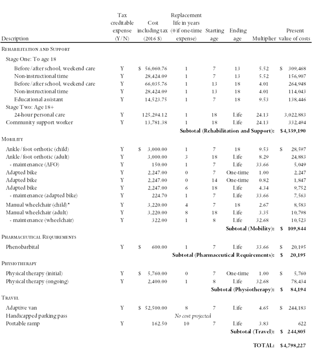
 * The cost of care expert recommended that the wheelchair be replaced approximately every three to five years. It was also indicated that once the child’s chair had reached its maximum capacity, it would have to be replaced with an adult chair. For the purposes of our calculations, we have assumed that the chair will require replacement every four years until the plaintiff is eighteen.

We would like to thank Stephen Kuyltjes of Rehab Works, Calgary; Sharon Kaczkowski of Kaczkowski Occupational Therapy, Calgary; and Everett Dillman of International Business Planners, El Paso, Texas, all of whom were kind enough to comment on earlier drafts of this article. We are responsible for any remaining errors or omissions.

leaf

Christopher Bruce is the President of Economica and a Professor of Economics at the University of Calgary. He is also the author of Assessment of Personal Injury Damages (Butterworths, 2004).

Kelly Rathje is a consultant with Economica and has a Master of Arts degree (in economics) from the University of Calgary.


The Effect of Incarceration on Future Earnings

by Christopher J. Bruce, Derek W. Aldridge

In personal injury and fatal accident claims, the courts are often required to determine what effect a criminal record would have had on the earnings of the plaintiff. We suspect that most individuals would expect that criminals will have lower wages and higher unemployment rates than the average citizen.

In this paper, we summarise the most reliable research that has been conducted into this question. We divide this summary into four lines of investigation: the impact of incarceration on earnings and employment; the effect of an increase in the duration of incarceration; the determinants of a successful transition from jail to civilian life; and the determinants of the probability of recidivism.

Incarceration

Although the raw data indicate that those who have been incarcerated have lower earnings and higher unemployment rates than those who have no criminal record, research indicates that this is an example of “correlation, not causation.” (For further information on the misuse of statistics in legal proceedings, see Bruce, 2004.) That is, careful analysis of the data have shown that individuals with low earnings and high unemployment rates are more likely to commit (and be convicted of committing) crimes than are those with high earnings and low unemployment rates. Hence, the primary reason that earnings are low among those who have been incarcerated is that those individuals are drawn from a population of individuals who have low earnings, not because the incarceration changed their employment prospects.

Grogger (1995), for example, found that neither arrests nor jail terms had long term effects on the earnings or employment of young men. And Kling (1999) concluded that, for most individuals, incarceration only reduced earnings by 0 to 3 percent, five to eight years after release. The only group for whom incarceration had a significant effect on post-release earnings was white collar criminals (such as accountants and stockbrokers). Similarly, Richey (2015) found that the effect of conviction on earnings was small or zero. Western (2002), however, found that although conviction had no effect on employability, it reduced the rate of growth of earnings by approximately 33 percent. (Note, however, that as rates of growth are often approximately two or three percent per year, a 33 percent reduction implies a reduction in rate of growth of approximately one percent or less.)

Duration of incarceration

A number of recent articles have attempted to determine whether an increase in the length of a jail sentence, holding the severity of the crime constant, has an effect on post-incarceration employment and earnings. One study found that there “…. is no substantial evidence of a negative effect of incarceration length on employment or earnings.” (Kling, 2006) Another found that the length of prison sentence for drug offences had no significant effect on earnings; but that length of sentence had a very significant effect with respect to incarceration for fraud and embezzlement. (Lott, 1992)

Transition from prison into the workplace

A small number of studies have investigated the factors that influence the success of transition out of prison. Typical of these is Visher and Travis (2003) in which the authors found that men with close ties to families and friends made the most successful transitions into the workplace, particularly if they lived with their wives and children. Families appeared to be especially important if they provided emotional support and housing assistance.

Recidivism

Numerous studies – e.g. Gendreau et. al. (1996), Jones (2005), and Motiuk and Vuong (2005) – have concluded that those who have been released from prison are more likely to reoffend if they have experienced high levels of unemployment or job instability, lack a skill or trade, or are drug users. They are also more likely to reoffend the younger they are.

The finding that it is younger individuals who are most likely to re-offend implies that most offenders have left the criminal population by the time they are in their late 20s. One Canadian study (Correctional Service of Canada, 1993), found that, at age 32, the average age at which respondents had committed their last offence was 23. A subsequent study (Ouimet and LeBlanc, 1996), based on interviews with 238 young men who had previously been young offenders, found that whereas more than half had been criminally active between the ages of 18 to 25, only 18 percent had been criminally active after 25.

Summary

The scientific literature suggests that incarceration has a relatively small effect on lifetime earnings. Although those who have been incarcerated earn lower incomes than those who have not been incarcerated, it is primarily because they are drawn from a group that tends to have relatively low earnings, not because the incarceration “causes” low earnings. Further, the data appear to indicate that the likelihood of being convicted and sent to jail decreases as an individual ages. Hence, those 30 and 40 year olds who were incarcerated in their early 20s are not likely to become repeat offenders.

It appears, therefore, that once a plaintiff reaches the age of approximately 25, the best predictors of his future earnings are standard factors like earnings history, education, and occupation. Whether or not that individual has been incarcerated will not add a significant amount of information to the factors that are used to forecast earnings of non-incarcerated individuals.

Sources

  • Bruce, Christopher, (2004) “The Reliability of Statistical Evidence Concerning the Impact of Disability;” Expert Witness, 9(4), http://www.economica.ca/ew09_4p1.htm.
  • Correctional Service of Canada, (1993) “Recidivists tend to be…;” Forum on Corrections Research, 5(3).
  • Gentreau, P. et. al. (1979) “Norms and recidivism for first incarcerates: Implications for programming;” Canadian Journal of Criminology, 1-26.
  • Grogger, J. (1995) “The effect of arrests on the employment and earnings of young men;” Quarterly Journal of Economics, 51-71.
  • Jones, D. (2005) “Offender employment: A research summary;” Forum on Corrections Research, 17(1), 13-20.
  • Kling, J. (1999) “The effect of prison sentence length on the subsequent employment and earnings of criminal defendants;” Woodrow Wilson School Discussion Papers in Economics.
  • Kling, J (2006) “Incarceration length, employment, and earnings;” American Economic Review, 863-876.
  • Lott, J (1992) “Do we punish high income criminals too heavily?;” Economic Inquiry, 583-608.
  • Motiuk, L, and B. Vuong (2005), “Offender employment: What the research tells us;” Forum on Corrections Research, 17(1), 21-24.
  • Ouimet, M., and M. LeBlanc (1996) “Life events in the course of the adult criminal career;” Criminal Behavior and Mental Health, 6(1), 75-97.
  • Richey, J. (2015) “Shackled labor markets: Bounding the causal effects of criminal convictions in the U.S.;” International Review of Law and Economics, 41, 17-24.
  • Visher, C., and J. Travis (2003) “Transitions from prison to community: Understanding individual pathways;” Annual Review of Sociology, 29, 89-113.
  • Western, B. (2002) “The impact of incarceration on wage mobility and inequality;” American Sociological Association, 4, 526-546.

leaf

Christopher Bruce is the President of Economica and a Professor of Economics at the University of Calgary.

Derek Aldridge is a consultant with Economica and has a Master of Arts degree (in economics) from the University of Victoria.

Spring 2016 issue of the Expert Witness newsletter (volume 20, issue 1)

Contents:

This issue contains two articles written by Dr. Christopher Bruce. The first reviews the debate over the use of cross versus sole dependency approaches in the determination of loss of dependency on income; while the second article concerns the reliability of income data drawn from the 2011 census.

Cross versus Sole Dependency in Fatal Accident Actions

  • In the first article, Dr. Bruce notes that a fundamental assumption in economics is that individuals are rational. Therefore, when an individual is observed to make a voluntary choice, it can be concluded that the individual must have expected that choice to make him/her better off (or at least, no worse off). With respect to fatal accident actions, this implies that if spouses are rational, they must have expected that the decisions they made about spending on one another would make them better off. He then shows that if this proposition is accepted, the sole dependency approach is preferred to cross dependency.

Are Data from the 2011 Census Reliable?

  • In the second article, Dr. Bruce examines the reliability of the 2011 Census income data. In the past, completion of the long form census was mandatory. In 2011, however, completion of this form was voluntary and the response rate decreased. While this created statistical problems concerning the reliability of the data, Statistics Canada had anticipated these problems and took steps to mitigate them. In his article, Dr. Bruce discusses these problems, and the solutions implemented by Statistics Canada, concluding that the 2011 census remains a reliable, high quality data source. It will remain our primary source of earnings information until data from the 2016 census are released sometime in 2018.
  • With respect to the 2016 census, we would note that it will be mandatory. Further, Statistics Canada will be sending the long-form section to a greater number of households than in past censuses (one in four households instead of one in five households), and will use income data directly from the Canada Revenue Agency, providing data for 100 percent of households. It is anticipated that because of these changes, the income data from the 2016 census will be the most accurate of any census to date.

A Pdf. version of the newsletter can be found here.

Are Data from the 2011 Census Reliable?

by Christopher J. Bruce

When estimating future earnings in personal injury and fatal accident cases, financial experts often rely on information provided by the Canadian Census. Of particular importance are data concerning incomes by age, sex, occupation, and education. For example, if a 24 year-old male plaintiff would have been a journeyman carpenter, his potential earnings might be based on average incomes for Canadians with that certification, in the age groups 25-29, 30-34, 35-44, etc.

In the past, these data would have been drawn from a section of the Census known as the “long form.” This portion of the Census survey, which contained much more detailed information than on was on the rest of the Census, was given to only one household out of five. (The remainder of the Census survey asks only basic questions about such demographic factors as age, sex, language, and area of residence.)

For the 2011 Census, however, the government decided to replace the long-form questions with a “National Household Survey (NHS).” Although the 2011 NHS asked the same questions as had the 2006 Census long form, whereas the long form had been mandatory, the NHS was voluntary. The result, as had been expected, was that the percentage of households answering this portion of the survey fell significantly, from 93.8% in 2006 to 77.2% in 2011.This created three statistical problems concerning the reliability of the data (variability in small community data, sample error, and non-response bias). As Statistics Canada had anticipated these problems, however, it took steps to mitigate them, steps that have maintained the reliability of the data that are of value to the courts. Wayne R. Smith, Chief Statistician of Canada, recently wrote an article in which he discussed these steps. [“The 2011 National Household Survey – the complete statistical story,” http://www.statcan.gc.ca/eng/blog-blogue/cs-sc/2011NHSstory. June 4, 2015.] In this article, I summarise Dr. Smith’s discussion.

Variability in small community data

As the sample size of any survey becomes smaller, the data become less and less reliable, due to an increase in variance. In response, Statistics Canada routinely withholds data concerning the smallest communities. In 2011, they withheld the results from 1,100 such communities, up from 160 in the 2006 Census. That is, all of the data reported in 2011 meet the normal statistical requirements for reliability.

Sample error

As the overall size of a sample decreases, there is an increase in what is known as the “sampling error;” that is, from the problem that the average characteristics of the sample differ from the average of the total population. Because Statistics Canada expected a smaller percentage of households to answer the voluntary NHS than had answered the mandatory long form, they anticipated that the total size of the “sample” (the households answering the survey) would be lower in 2011 than in 2006.

To deal with this problem, Statistics Canada increased the number of households who were asked to answer the long portion of the 2011 Census. Whereas one household in five were asked to answer the 2006 long form, one household in three were asked to answer the NHS. The result was that, even though a smaller percentage of households responded to the NHS than had responded to the 2006 long form, the number of households answering the NHS was higher than in 2006, (2,657,461 versus 2,443,507, representing 6,719,688 versus 2006’s 6,136,517).

Although this approach does not correct for all errors, those errors become less and less important as the data are aggregated. Thus, for example, the data for the average income of all carpenters in Alberta are more reliable than for the average income of carpenters in Calgary.

Non-response bias

The most worrisome problem that arises when a survey is made voluntary is that the households who choose to respond to that survey may differ significantly from those who refuse to do so. For example, if those carpenters with relatively high incomes are more likely to respond to the NHS than are those with low incomes, the average incomes reported by the NHS will be biased upwards.

Statistics Canada could not control, ex ante, for the possibility that this would happen. However, they were able, ex post, to investigate whether the respondents to the NHS were representative of the overall groups from which they were drawn – that is, they were able to determine whether the respondents “looked” different from the average.

To make this determination, Statistics Canada was assisted by the fact that they had a considerable amount of information about the respondents to the NHS before those individuals answered the NHS survey. Most importantly, they also had their responses to the short questions on the Census that are mandatory for all Canadians. In addition, they were also able to link the NHS respondents to those individuals’ tax files, immigrant landing data, and the Indian Register.

Using sophisticated statistical techniques they were able to determine that the average respondent to the NHS had very similar characteristics to the average Canadian with respect to age, sex, language, area of residence, income tax, immigration status, and aboriginal status. This finding leads Statistics Canada to conclude that the NHS respondents were, in most cases, representative of the larger population from which they were drawn. And when Statistics Canada was unable to conclude that the individuals who replied to a specific sub-class of questions were representative of the population, the resulting data were not released, or they were released with an accompanying cautionary note.

Summary

To summarise: Although the long-form portion of the 2011 Census was made voluntary, there is sound reason to believe that the data that are of greatest relevance to the calculation of lost earnings can be relied upon.

  1. The information in this article is drawn from a blog written by Wayne R. Smith, Chief Statistician of Canada, entitled “The 2011 National Household Survey – the complete statistical story,” June 4, 2015. This blog can be found at: http://www.statcan.gc.ca/eng/blog-blogue/cs-sc/2011NHSstory.


Christopher Bruce is the President of Economica and a Professor of Economics at the University of Calgary. He is also the author of Assessment of Personal Injury Damages (Butterworths, 2004).

Cross versus Sole Dependency in Fatal Accident Actions

by Christopher J. Bruce

When a spouse has been killed through the negligence of a third party, the surviving spouse is entitled to damages that would allow him/her to maintain the standard of living that he/she had previously enjoyed.

The determination of this value requires that three steps be taken. First, the potential earning capacity of each spouse must be estimated. Second, a calculation must be made of each spouse’s dependency rate – that is, the percentage of family income that benefitted that spouse. Third, it must be determined whether any monies that had been spent on the deceased by the survivor (and which now do not have to be spent due to the death of the former) should be deducted from the survivor’s loss of dependency. In what is known as the sole dependency approach, that “saving” is not deducted. In the cross dependency approach, the saving is deducted.

In this article, I will use a concept that is fundamental to economic analysis – the rational person assumption – to suggest that basic economic principles favour the use of sole dependency.

I begin by making some simple assumptions about a couples’ earning capacity and dependency rates and use those assumptions to define sole and cross dependency. I then introduce the rational person assumption and provide examples of the use of that assumption in non-fatal accident cases. Finally, I extend the analysis to fatal accident cases and argue the rational person assumption provides support for use of the sole dependency approach.

Assumptions concerning earning capacity and dependency

Statistical analyses suggest that, in a household consisting of a husband and wife, approximately 30 percent of the family’s after-tax income is spent on items such as food, clothing, and transportation that benefit the husband alone; approximately 30 percent is spent on items that benefit the wife alone; and 40 percent is spent on items, such as housing, furniture, and insurance, that benefit both spouses collectively. Each spouse benefits, in total, from 70 percent of family income – 30 percent that benefits that spouse personally – usually referred to as “personal expenses” – and 40 percent that benefits both spouses equally – “common expenses.” The 70 percent figure in this example is known as the individual spouse’s “dependency rate.” [Note that, as both spouses have the same dependency rate, 70 percent, there is a net benefit from marriage.]

Assume that in a childless couple, the husband earns $100,000 per year after taxes and the wife earns $40,000. Based on my assumptions concerning dependency rates, out of the husband’s income, 30 percent, or $30,000, is devoted to his personal expenses, 30 percent, or $30,000, is devoted to his wife’s personal expenses, and 40 percent, or $40,000, to common expenses. From the wife’s income, the comparable figures are 30 percent ($12,000), 30 percent ($12,000), and 40 percent ($16,000), respectively.

Cross and sole dependency defined

Now, assume that the wife has been killed. The sole dependency approach asks: how much of the wife’s future income would have been devoted to expenses that benefitted the husband? The answer in this case is that it is the 30 percent of her income that she spent on items specific to her husband (food, clothing, etc.) plus the 40 percent of her income that she spent on common expenses (housing, furniture, etc.), or $28,000 – which equals the husband’s dependency rate, 70 percent, multiplied by the wife’s (after-tax) income, $40,000. The tortfeasor would be required to pay $28,000 per year until the projected date of the wife’s retirement, discounted to the present.

Proponents of the cross dependency would also calculate the husband’s dependency on the wife’s income, here $28,000. But they would then argue that there is an offset against that loss: the “savings” obtained by the husband because he no longer devotes 30 percent of his income to his wife’s personal expenses. In the example here, as the husband was spending 30 percent of his income on his wife, it is argued that he now benefits from a $30,000 saving as a result of her death. The difference between this $30,000 saving and the $28,000 he has lost, $2,000 per year in total, represents a net benefit to him. He has no claim (for dependency loss) against the tortfeasor.

The “Rational Person” assumption

Which of these approaches is more consistent with the legal principal that plaintiffs are to be returned to the position they would have been in had the negligent action not occurred, restitutio in integrum?

When answering this question, economists rely on an assumption that is fundamental to economic analysis: that individuals act rationally to improve their own welfare. This rational person assumption implies that informed individuals will voluntarily undertake actions only if those actions make them better off (or, at least, no worse off). [Note the similarity to the “reasonable person” doctrine of tort law and to the rationale, in contract law, for maintaining the sanctity of contracts.]

As a simple example of the rational person assumption, assume that individual B is observed to be saving towards the purchase of a lap-top computer. One day, B sees an ad for the computer he likes, at a price of $1,000 (inclusive of all taxes). He checks his bank balance and discovers that he has $1,500. Assume we also observe him use his debit card to buy the desired computer; and, when he gets home, to check his bank balance again, to find that he now has $500.

Can we, as an external observer (with no ability to read B’s mind) conclude that B is “better off?” Economists, employing the “rational person” assumption, argue that B must be better off than if the purchase had not been made: a rational individual will only pay $1,000 for an item if he or she values that item at more than (or equal to) $1,000.

Although it might be argued that B is “worse off” in the sense that he now has $1,000 less than he would have had, that reduction in his finances is at least offset by the fact that he now has a computer that he valued at $1,000 or more.

To put it another way, if an individual was observed to go shopping with the intention of paying $1,000 for a computer, but was prevented from doing so because the store had run out of stock, no professional economist would argue that that individual was now “better off” — because he now has $1,000 that he would otherwise not have had. He is not better off. His preference was observed to be to trade the $1,000 for a computer – that would have made him better off. [Indeed, the rational person assumption suggests that when he is prevented from spending his money the way that he prefers, he is made worse off.]

The Rational Person argument applied to personal injury cases

Before examining how this view of rational behaviour applies to fatal accident cases involving spouses, I first turn to two other classes of tort actions.

In the first of these actions, assume that an individual has been seriously injured in a motor vehicle accident. As a result of this accident, her earning capacity has been impaired to the extent that she will lose $100,000 between now and the time she would have retired. The defendant accepts responsibility for this loss, but counters that offset against this loss is a “gain” that the plaintiff has obtained because of the accident. Imagine that before the plaintiff was injured, she was an active golfer, spending $5,000 a year on green fees, lessons, and equipment. The injuries suffered in the accident, however, are such that she can no longer play golf, thereby “saving” $5,000 per year. Assume also that evidence has been led to suggest that she would have played golf for another 25 years, had she not been injured. Hence, because of her injuries, she will save approximately $125,000 over her lifetime that would otherwise have been spent on golf. The defendant argues that when this saving is deducted from the plaintiff’s lost earnings, the plaintiff is actually $25,000 better off as a result of the accident. The defendant owes nothing to the plaintiff.

Using the assumption of the rational individual, however, it is easily seen why the defendant’s argument in this case is fallacious. Although it is true that the plaintiff will now have $125,000 available to her that she would not have had in the absence of the accident, she now has been denied $125,000 worth of pleasure that golf would have given her. Ignoring the effect of the accident on her earnings, in order for the plaintiff to be left in the same position she would have been in the absence of the accident, she will have to spend sufficient money to replace the value she would have obtained from golf. But this must be at least $125,000: because she would have chosen to spend $5,000 per year on golf in preference to spending it on anything else, $5,000 spent on “anything else” must be of lesser value than that expenditure on golf. That the plaintiff now has $125,000 that she would not have had if she had been allowed to spend it on golf does not make her $125,000 better off. At best, it leaves her in approximately the same position as she would have been in had she been allowed to spend that money. Hence, it is incorrect to suggest that the $125,000 that has been “saved” should be set off against the plaintiff’s loss of earnings.

In the second example of a tort action, assume again that the injuries suffered by the plaintiff in an automobile accident have reduced his lifetime earnings by $100,000. Again, the defendant has accepted responsibility for the accident; but in this case, she argues that as the plaintiff’s daughter was killed in that accident, the plaintiff has been “saved” the costs of raising that child. If those costs have been calculated to be $150,000 over the life expectancy of the child, the defendant argues that the net effect of the accident has been to leave the plaintiff no worse off than he had been in the absence of the accident. There is no loss.

Again, the fallacy of this argument arises because the defendant has implicitly argued that the plaintiff would not have received any benefit from the $150,000 he would have spent on his daughter. But, according to the “rational consumer” assumption, if the plaintiff had chosen to have the daughter and to spend $150,000 on her, in preference to spending that money in any other way, the plaintiff is worse off having $150,000 than he would have been spending that money on his daughter.

The Rational Person argument applied to fatal accident cases

With these cases in mind, consider again the case discussed at the beginning of this article, concerning the death of a wife. It is now seen that when the defendant argues that the cross dependency approach should be applied, what he is actually arguing is that the $30,000 the plaintiff had been spending on his wife had provided him with no benefit at all. Now that those expenditures have been “freed up”, he can spend the money on himself, at a net gain of $30,000. Therefore, the defendant argues that that gain can be set against other losses from the accident – as was argued by the defendants in the cases of the plaintiffs who were asked to set their savings of expenditures on golf or on their child against their losses of income.

But, as in those cases, the rational person assumption suggests that surviving spouses are not better off when they do not “have to” make expenditures on their deceased partners. If they were making those expenditures voluntarily (i.e. rationally), they must have obtained some benefit from that expenditure – indeed, a benefit that exceeded the value from any other purchases that could have been made with the same amount of money. Now that the husband in the example does not “have to” spend $30,000 per year on his wife, he can spend it on himself – clothes, travel, cars, etc. But does that expenditure give him as much pleasure as spending it on his wife? The better argument, I suggest, is that preventing plaintiffs from spending money in the way that they would have chosen cannot make them better off. Hence, it would be inappropriate to deduct any such purported “gains” from plaintiffs ‘other losses.

It is the sole dependency approach that is more consistent with both restitutio in integrum and with the rational person assumption.

Summary

A fundamental assumption in economics is that individuals are rational; and, therefore, that when an individual is observed to make a voluntary choice, it can be concluded that the individual must have expected that choice to make him/her better off (or, at least, no worse off). With respect to fatal accident actions, this implies that if spouses are rational, they must have expected that the decisions they made about spending on one another would make them better off. In this article, I have argued that if this proposition is accepted, the sole dependency approach is preferred to cross dependency.


Christopher Bruce is the President of Economica and a Professor of Economics at the University of Calgary. He is also the author of Assessment of Personal Injury Damages (Butterworths, 2004).