Winter 2004/05 issue of the Expert Witness newsletter (volume 9, issue 4)

Contents:

  • The Reliability of Statistical Evidence Concerning the Impact of Disability
    • by Christopher Bruce
    • In the article Christopher Bruce provides a caution concerning the acceptance of statistical evidence about disability. Dr. Bruce argues that the courts and opposing counsel do not subject certain types of medical opinion to sufficiently strict statistical standards. Specifically, he shows that evidence based on: (i) the expert’s “experience,” (ii) the expert’s interpretation of third party statistics, or (iii) the expert’s understanding of published statistical reports may be unreliable. In this article, he provides examples of how statistical evidence may fail to meet the standards expected by the courts; and he offers suggestions about how counsel might respond to these deficiencies.
  • Statement of Ethical Principles and Principles of Professional Practice – National Association of Forensic Economics
    • Economica belongs to an organization of forensic economists known as the National Association of Forensic Economists (NAFE). NAFE has recently published a “Statement of Ethical Principles, and Principles of Professional Practice.” As Economica subscribes to the principles outlined in the NAFE Statement, we have reproduced it here.

Statement of Ethical Principles and Principles of Professional Practice – National Association of Forensic Economics

This article first appeared in the winter 2004 issue of the Expert Witness.

The National Association of Forensic Economics (NAFE, nafe.net) has members – including Economica – across the United States and internationally. It publishes the Journal of Forensic Economics which contains articles of interest to economists, accountants, finance and business professionals, vocational counselors, lawyers, and actuaries engaged in such fields as business valuation, commercial litigation, employment litigation, and personal injury and wrongful death torts.

NAFE also sponsors programs at regional and national economic conferences and has its own Winter and International meetings. Additionally, members communicate via an internet mailing list and quarterly newsletters.

As a condition of membership, members pledge to adhere to NAFE’s Statement of Ethical Principles and Principles of Professional Practice. We reproduce the statement below.


When providing expert opinion for use as evidence by the trier of fact, a NAFE member pledges, as a condition of membership, adherence to the following:

1. Engagement

Practitioners of forensic economics should decline involvement in any litigation when they are asked to assume invalid representations of fact or alter their methodologies without foundation or compelling analytical reason.

2. Compensation

Practitioners of forensic economics should not accept contingency fee arrangements, or fee amounts associated with the size of a court award or out-of-court settlement.

3. Diligence

Practitioners of forensic economics should employ generally accepted and/or theoretically sound economic methodologies based on reliable economic data. Practitioners of forensic economics should attempt to provide accurate, fair and reasonable expert opinions, recognizing that it is not the responsibility of the practitioner to verify the accuracy or completeness of the case-specific information that has been provided.

4. Disclosure

Practitioners of forensic economics should stand ready to provide sufficient detail to allow replication of all numerical calculations, with reasonable effort, by other competent forensic economics experts, and be prepared to provide sufficient disclosure of sources of information and assumptions underpinning their opinions to make them understandable to others.

5. Consistency

While it is recognized that practitioners of forensic economics may be given a different assignment when engaged on behalf of the plaintiff than when engaged on behalf of the defense, for any given assignment, the basic assumptions, sources, and methods should not change regardless of the party who engages the expert to perform the assignment. There should be no change in methodology for purposes of favoring any party’s claim. This requirement of consistency is not meant to preclude methodological changes as new knowledge evolves, nor is it meant to preclude performing requested calculations based upon a hypothetical – as long as its hypothetical nature is clearly disclosed in the expert’s report and testimony.

6. Knowledge

Practitioners of forensic economics should strive to maintain a current knowledge base of their discipline.

7. Discourse

Open, uninhibited discussion is a desired educational feature of academic and professional forensic economic conferences. Therefore, to preserve and protect the educational environment, practitioners of forensic economics will refrain from the citation of oral remarks made in an educational environment, without permission from the speaker.

8. Responsibility

Practitioners of forensic economics are encouraged to make known the existence of, and their adherence to, these principles to those retaining them to perform economic analyses and to other participants in litigation. In addition, it is appropriate for practitioners of forensic economics to offer criticisms of breaches of these principles.

The Reliability of Statistical Evidence Concerning the Impact of Disability

by Christopher Bruce

This article first appeared in the winter 2004 issue of the Expert Witness.

Expert witnesses often testify that their experience, or the latest research, leads them to believe that a plaintiff’s injuries will have certain long-term physical, educational, or employment consequences. For example, the plaintiff’s injuries are predicted to worsen, or improve, along some projected time line. Or those injuries are expected to affect the probability that the plaintiff will be able to complete a planned educational program or enter a preferred occupation. Or an opinion will be given concerning the effect that certain disabilities will have on the income that the plaintiff will be able to earn.

When listening to such testimony, I am often reminded of Benjamin Disraeli’s famous complaint that “there are three kinds of lies: lies, damn lies, and statistics.” Expert testimony – particularly expert testimony with respect to the application of medical statistics to the determination of damages in personal injury cases – gives rise to three alternative interpretations that might be attached to Disraeli’s adage.

First, there is the sense in which I suspect Disraeli himself meant his quote: as a complaint that laypeople – judges and lawyers in this case, politicians in his – often find the (statistical) testimony of expert witnesses to be so confusing that they have difficulty distinguishing fact from fiction. That is, his was a call for more clarity; less use of obscure, technical language.

A second version might be recast as: there are “liars, damn liars, and those who abuse statistics.” This is a complaint against those who intentionally twist the interpretation of statistics, hoping either that the opposing expert has insufficient statistical knowledge to be able to recognise the deception, or that the court will have insufficient expertise to be able to determine which of the experts is telling the truth.

Finally, the sense in which Disraeli’s dictum is of greatest relevance to legal advocacy might be restated as: there are “liars, damn liars, and those who misuse statistics.” By this I mean the situation in which “experts” have insufficient knowledge of statistical analysis to realize that they have misunderstood or misrepresented the data that they are citing. My experience suggests both that this situation occurs with depressing frequency in personal injury cases, particularly with respect to medical statistics; and that opposing counsel allow these “misused” statistics to go unchallenged far too often.

The purpose of this paper will be to assist the courts to recognise the sources of statistical “misuse” and to institute methods of responding to the errors that arise. In a second paper, to be published in the next issue of the Expert Witness, I will report a number of statistics concerning the impact of disabilities on earning capacity, taken from sources that use reliable statistical techniques.

Sources of Statistical “Misuse”

There are three reasons why statistical evidence concerning the impact of disabilities on earnings might not be reliable. First, the expert may be basing his/her conclusions on past experience treating patients similar to the plaintiff, without taking into account the statistical uncertainties inherent in such an approach. Second, the expert, due to inadequacies in his or her own statistical training, may have misinterpreted data produced by a third party. Third, the expert may not have recognised that the data he or she is using to develop a prognosis were themselves collected or reported using unreliable statistical techniques. Examples of each of these types of error are discussed in this section.

1. The Expert’s Experience May Not Be Reliable

In many cases, experts drawn from the specialties that treat plaintiffs’ injuries – doctors, psychologists, physiotherapists, etc – rely upon their past experiences dealing with patients similar to the plaintiff to predict the impact that the plaintiffs’ injuries will have on his/her future ability to earn income. There are many reasons why the court should be reluctant to rely on this experiential evidence:

1. The plaintiff may not be representative of the patients that the medical expert normally treats: thus, the expert’s experience may not transfer easily to the plaintiff’s situation. For example, if the expert lives in a large city and the plaintiff comes from a rural area, the expert may not be familiar with the impact that a particular type of injury will have on the plaintiff’s ability to work on a farm. Or if the expert normally treats working-age patients, he/she may not be familiar with the impact of a particular type of disability on a senior or a minor.

2. If the medical expert has treated only a small number of individuals like the plaintiff, the sample size may be too small to draw statistically reliable inferences. For example, even a doctor who specialises in spinal cord injuries may have treated only a small number of quadriplegics. His/her experience with such a small number will provide only limited information concerning the plaintiff.

3. Even if the medical expert has treated a relatively large number of individuals like the plaintiff over his/her career, if the recommended treatment for those individuals has changed significantly recently, the expert may have treated only a small sample since that change. Again, the number of patients receiving the new treatment may not be sufficient to draw reliable inferences.

4. Often, the medical expert has been asked to comment on the impact that a disability has on employment, schooling, or earnings. As these are non-medical outcomes, the expert may not have systematically monitored them. Thus, the sample on which his/her information is based may be biased. For example, those patients who have adjusted well to their injuries, and who have returned to work, may be less likely to return to a doctor or psychologist for further treatment than those who have had difficulty adjusting. In this case, the doctor/psychologist may have developed an overly pessimistic view of the effects of the injury.

5. If the harm to the plaintiff is expected to continue for decades into the future and the medical expert has not been in practice long enough to have experience with patients whose treatment has continued for that length of time, the expert’s experience may not be reliable for predicting long-term consequences.

2. “Expert” Interpretation of Statistical Studies May Not be Reliable

When the expert attempts to supplement information drawn from his/her own experience with information drawn from studies conducted by third parties, a new set of problems arises. Specifically, the expert may lack sufficient knowledge or experience to be able to interpret statistical studies correctly:

1. The expert may have insufficient experience in the field to recognise deficiencies in the data. Many medical studies, for example, use a definition of “unemployment” that differs from that which is used by agencies such as Statistics Canada. The unsuspecting reader, who tried to compare the statistics drawn from the former with those drawn from the latter, could reach erroneous conclusions. Indeed, even within a reliable agency, such as Statistics Canada, similar-sounding names are often used to refer to quite different concepts. One must be careful, for example, to distinguish between “constant” and “current dollar” wages, between “net” and “gross” income, and between “real” and “nominal” interest rates. Failure to recognise these differences can lead to serious errors.

2. Because there is a lack of reliable data for predicting the effects of disability on labour market outcomes, experts are often forced to rely on data that were collected for other purposes. In many cases, this leads to the inappropriate use of such data. For example, doctors often use the American Medical Association “Guides to the Evaluation of Permanent Impairment” to calculate an index of the percentage of “whole body function” that has been lost due to an injury. Loss of an eye, for example, might be considered to reduce the patient’s “whole body” physical capacity by 25 percent.

Although the AMA did not design this index as a method of predicting the impact of disability on earnings, in the 1960’s and 1970’s it became common for experts to argue that a 25 percent reduction in whole body functioning implied a 25 percent reduction in earning capacity. Yet the connection between, say, loss of an eye or loss of a foot on the one hand, and loss of earnings capacity on the other is a tenuous one at best. Whereas loss of an eye could end the career of a professional athlete, for example, it might have very little impact on the career of an economist or lawyer.

Similarly, the rating system developed by Statistics Canada to categorise disabilities as mild, moderate, or severe yields statistics that are of very little value for predicting the effect of disability on the earnings of individuals within specific occupations. Yet many experts are currently using these statistics to make predictions of this nature.

3. The expert’s training in statistical analysis may be insufficient to allow him/her to distinguish reliable studies from unreliable ones. For example, studies that attempt to draw a connection between disabilities and labour market measures (such as income and employment) commonly rely on unsophisticated statistical techniques, making their conclusions very unreliable. Expert witnesses who are not well trained in statistical analysis may be unable to distinguish reliable studies from unreliable ones.

3. Published Studies May Not be Reliable

The most important problem facing the expert who wishes to predict the effect that disabilities will have on earning capacity is that many (if not most) of the statistical studies that have been published on this topic are unreliable. Some of the most important problems of which the courts should be aware include:

1. Many studies of the impact of disability on employment rely on very small samples. For example, it is not uncommon for articles on medical issues to study as few as 10 or 20 patients. Yet it is well known to statisticians that, in order to avoid the problem that “outliers” will bias statistical findings, it is usually necessary to have hundreds of observations.

2. Before the findings from a survey can reliably be projected to the population in general, it is crucial to ensure that the survey group is chosen in such a way as to be representative of the “population.” Many medical studies survey the patients from a single hospital or clinic, for example. But the findings of such a survey cannot reliably be projected to the general population if that hospital or clinic draws only from a sub-set of the population – for example, only from a relatively wealthy district or only from an urban population. And studies that attempt to contact patients many years after treatment may be biased in the sense that it may be easier to locate certain sub-sets of the group than others. For example, those paraplegics who have had the greatest success adjusting to their condition may be the ones who are most likely to have moved from the addresses they had at the time of admission to hospital and, therefore, may be the most difficult to reach at the time of the survey.

3. Although there are multiple factors that influence the effect of disability on employment and earnings, studies often collect information on only a small sample of these factors. For example, if older individuals are more likely to suffer from a particular disability (like arthritis) than are younger individuals, a data set that did not provide information about the ages of the individuals surveyed might appear to suggest that individuals with that disability earn higher average incomes than those who are not disabled (because individuals’ incomes tend to rise with age). Similarly, studies may overestimate the impact of a disability if more low-income than high-income individuals suffer from that disability.

4. Statistical studies can only show that variables – for example, disability and earnings – are correlated: they cannot show that one “causes” the other. That is, it is not clear whether disability causes low earnings, or whether occupations with low earnings have high accident rates. Labourers, for example, are more likely to experience on-the-job accidents than are office workers. If office workers earn more than labourers, data may appear to suggest that job-related accidents “cause” a significant reduction in earnings “because” those who have been injured earn less than the average person in the population. The more appropriate interpretation may have been that it was low income that had “caused” the accidents – that is, that it was the occupations with low earnings that had high accident rates.

One of the most common problems with medical studies is that they often do not report the age at which the disability became apparent. Yet we would expect that loss of a leg or an eye would affect individuals’ earnings differently if they were injured before they had completed their educations than if they were injured after they had established their careers.

What Can Counsel Do?

Medical experts often go unchallenged by the courts, even when they use unreliable statistical methods. How can the courts circumvent this problem, given that most lawyers and judges lack the expertise to question the bases of statistical testimony? I recommend three approaches:

1. If the opposing expert appears to be relying on his/her own experience as the basis for his/her predictions, at the “qualification” stage counsel should question the expert’s training in statistics. Do this not (necessarily) with the intention of convincing the court to reject his/her credentials, but to prepare the expert to agree with counsel that certain standards of data collection are important. Then use that agreement later to induce the expert to concede that his/her experience is inadequate for drawing reliable inferences.

2. Hire an expert in statistical analysis. Of those professions most commonly seen in court, actuaries and economists generally have the best training in advanced statistical techniques. Actuaries will have greater experience with life expectancy and fringe benefit data; while economists will have greater experience with data concerning education and incomes.

Other professions that also receive advanced statistical training are epidemiologists (often employed by medical schools) and statisticians (found in university departments of mathematics).

3. One option that is used occasionally in Canada, but less often than is justified, is to hire an expert in statistics to conduct original statistical analyses. As such an analysis is likely to cost at least $10,000-$20,000, it can not be justified for small, or “one-off” cases; but in a major injury case, in which the damages approach a million dollars, or with respect to the types of injury that counsel is likely to encounter many times, such an expenditure may well be justified. For example, my firm was hired by the defendants in one of the residential school sexual abuse cases. We used census data to estimate the earnings of individuals similar to the residents of those schools, but who had not been abused, and compared those earnings to the earnings of the plaintiffs. Similarly, in the second part of this paper (to be published in the next issue of the Expert Witness), I report the findings of a set of statistical analyses I conducted using Statistics Canada data, to determine the impact of various types of disabilities on educational attainment and income. These analyses could have been conducted by virtually any Ph.D.-trained economist in Canada.

leaf

Christopher Bruce is the President of Economica and a Professor of Economics at the University of Calgary. He is also the author of Assessment of Personal Injury Damages (Butterworths, 2004).

Autumn 2004 issue of the Expert Witness newsletter (volume 9, issue 3)

Contents:

  • Using family background to Predict Educational Attainment in Canada
    • by Carmen Anderson with Christopher Bruce
    • When a minor has suffered a serious injury, it is necessary to predict what the income level of the plaintiff would have been in the absence of that injury. In most cases, this is done by projecting an education level for the plaintiff and using census statistics to project the average income for that education level. This article examines some of the factors that can be used to predict a child’s eventual educational attainment.

Using family background to Predict Educational Attainment in Canada

by Carmen Anderson with Christopher Bruce

The article first appeared in the autumn 2004 issue of the Expert Witness.

Introduction

It is important, when predicting the lifetime income of a young plaintiff, to be able to identify the educational level that individual would have achieved, had he or she not been injured.

The economics literature contains numerous studies that have investigated the determinants of educational attainment. But all of these studies attempt to explain only tendencies in choice of education. Whereas they can tell us whether a minor is “more likely” to obtain post-secondary education if he or she comes from one socio-economic background than from another, they rarely attempt to predict the magnitude of these effects.

As a result, the literature is of only very general assistance to the court. In this article, we present the results of detailed statistical analyses we have undertaken, using a recent set of data compiled by Statistics Canada, that will allow us to provide more detailed predictions of educational attainment than have previously been available.

The Data

The data we employ, from the 2001 General Social Survey, allow us to compare the educational attainment of Canadians aged 30-39 with numerous characteristics from their family backgrounds.

Specifically, for each of approximately 5,000 survey respondents, we know whether the individual: failed to complete high school, completed high school, took “some” schooling beyond high school, completed a college diploma or trade certificate, or completed university. We have similar information for each of the respondent’s parents; and information about the respondent’s province of birth (or whether he/she was an immigrant), religion, and first language. We also know whether each respondent was an only child, whether the respondent lived with both of his or her parents while a child, and what size of city the respondent lived in when a child.

Table 1 presents a complete list of the variables available to us, along with their means and standard deviations. Notice that, with the exception of the education of the respondent at age 30-39, all the information presented in Table 1 would have been available when the individual was a teenager. Thus, if the respondent’s educational attainment is found to be correlated with that information, it may be possible to predict the ultimate education of individuals who are currently in their teens.

Table 1

Statistical Analysis

We subjected the data to a statistical technique known as regression analysis in order to determine which of the socio-economic variables were most closely correlated with educational attainment. We found that only three categories of variables had statistically significant effects. These were: the education of the parents, whether the individual lived with both of his or her parents until age 15, and (to a lesser extent) the population of the community in which the individual lived at age 15. Variables that proved to have no (or little) significant effect on educational attainment were: province of birth (if Canadian), whether the individual was an only child, immigration status, mother language, and religion.

Most importantly, we were able to use the results of our analyses to predict the probability that the respondent would achieve each of the five education levels, based on: parental education, whether the respondent lived with both parents until age 15, and the population of the community in which the respondent lived at age 15.

Parents’ Education

Tables 2 and 3 provide detailed information concerning the impact of parental education on the educational attainment of sons and daughters, respectively. As an example of how to read these tables, the top left box in Table 2 indicates that if both the mother’s and the father’s educations were less than high school (“< High School”), the probability that their son would also obtain less than high school education was 21 percent. The probability that he would finish high school was 24 percent, would finish “some” post-secondary schooling was 14 percent, would finish a trade or college education was 28 percent, and would finish university was 14 percent.

Table 2

Table 2 also indicates that, for males, the probability of completing the two “middle” levels of education – “some university or college” or
“college/trade school” – is not strongly influenced by parental education. For example, the probability of completing college or a trade varies only from 28 percent (when both parents had less than high school or had university) to approximately 34 percent (all other parents); and the probability of completing some college or university varies from 7 percent to 14 percent.

Similarly, Table 3 indicates that, for females, the probability of completing college or a trade varies only from 26 percent (when both parents had university) to 36 percent (most other parents); and the probability of completing some college or university varies from 5 percent to 15 percent (with a much smaller range if university educated parents are omitted).

Table 3

At either end of the educational range, however, parental education is a much more important predictor. When both parents have less than high school, for example, the probability that the child will complete high school or less is 42 percent for females (25 percent high school plus 17 percent less than high school) and is 45 percent for males; whereas when both parents have university educations, these probabilities fall to 5 and 8 percent, respectively.

Conversely, the probability that children will obtain university education rises from 13 percent for females and 14 percent for males, when both parents have less than high school, to 64 percent for females and 57 percent for males, when both parents have university degrees.

Furthermore, a one step change in parents’ education at either end of the educational range can have a dramatic effect on the child’s educational attainment. For example, whereas the probability that males would complete high school or less was 45 percent when their parents both had less than high school, that probability fell to 29 percent when their parents had completed high school.

And whereas the probability that females would complete university was 64 percent when both parents had also completed university, that percentage fell to 39 percent when both parents had college degrees or trade certificates.

Finally, it is important to note that the child’s educational attainment is influenced by the education of both parents. At most levels of education, an increase in the mother’s education has virtually the same effect on the child’s educational attainment as does an increase in the father’s education.

Lived with Both Parents

We were also able to use our statistical analyses to predict the effect that living with both parents had on individuals’ educational attainments. These predictions are reported in Table 4. There it is seen that, although living with both parents had a statistically significant effect on the child’s educational achievement, for practical purposes the impact is small. In particular, among both males and females, those who lived with both their parents were approximately 6 percent less likely to drop out of school before completing high school, and 9 percent more likely to complete university, than were those who lived with only one parent.

Table 4

Urban/Rural

Finally, Table 5 indicates that population of the area of residence makes very little difference to the educational decisions of females and has an important effect on the decisions of males only in very large cities, where males are approximately 10 percent more likely to attend university than are residents of smaller areas.

Table 5

Conclusion

Our results confirm earlier researchers’ findings that, in the prediction of the child’s educational attainment, virtually the only factor that is of importance is the education of the parents. Most importantly, the children of parents with less than high school education are much less likely to proceed beyond high school than are the children of parents at other educational levels. And the children of parents with university degrees are much more likely to complete university themselves than are the children of parents with lesser education.

Nevertheless, we also found that the education levels of the child’s parents were only indicative of a child’s educational attainment. The only situation in which 50 percent of the children of a set of parents had the same educational level as their parents (when both parents had the same education) was that in which both parents had university degrees. In every other case, it was rare for the probability that children would share their parents’ educational attainment to exceed 33 percent. This strongly suggests that, in the prediction of a child’s educational success, experts should generally present at least two (and, more often, three) alternative scenarios.

leaf

From 2003 until 2005, Carmen Anderson was a consulting economist at Economica, with a Master of Arts degree from the University of Calgary.

Christopher Bruce is the President of Economica and a Professor of Economics at the University of Calgary. He is also the author of Assessment of Personal Injury Damages (Butterworths, 2004).

Summer 2004 issue of the Expert Witness newsletter (volume 9, issue 2)

Contents:

  • The Impact of the “Net Income” Provisions of the Insurance Amendment Act, 2003
    • by Christopher Bruce
    • The article examines the implications of the changes to section 626.1 of the Insurance Act that were introduced in The Insurance Amendment Act, 2003. Dr. Bruce argues that these changes will: (i) require that income taxes be calculated for every year of both the with-accident and without-accident income streams in all personal injury cases; and (ii) raise the strong possibility that the courts will allow income tax “gross ups” on awards for loss of earnings. He also shows how the income tax gross up is calculated and estimates the overall impact of the revisions on personal injury awards; and he argues that those revisions will have no effect on the manner in which CPP premiums have been treated in Alberta.
  • Addendum: Calculating After-Tax Income Using Tables on Diskette

Addendum: Calculating After-Tax Income Using Tables on Diskette

by Hugh P. Finnigan

This article first appeared in the summer 2004 issue of the Expert Witness.

The Insurance Amendment Act, 2003 mandates that any loss of income award must be reduced by income tax. The purpose of this addendum is to introduce the reader to Tables on Diskette (TOD), a software program provided free of charge by the Canada Revenue Agency that can be used to calculate an individual’s net income (or after-tax income). That is, one can use TOD to estimate the Canada Pension Plan (CPP); Employment Insurance (EI); and federal, provincial (except Quebec) and territorial tax deductions, based on an individual’s gross earnings. The resulting net income figure can be incorporated into a loss of income estimate that is consistent with the provisions of the amended Insurance Act.

Installing the Software on Microsoft Windows

The latest version of TOD can be obtained from the Canada Revenue Agency’s website: www.cra-arc.gc.ca/tax/business/tod. To install the software,

  • Left-click on the link “Install.exe” located half-way down the web page (under the heading “How to download the “install” file to install TOD.” (Note: If you have a choice, it is better to use Internet Explorer for this purpose than Netscape Navigator.)
  • Select “Open” from the file download dialog box.
  • Once the file has decompressed, choose your language preference and select “OK.”
  • Read the introduction page and click “Next.”
  • Select the destination folder into which you would like to install TOD (or simply click “next” to accept the default).
  • Select where you would like the program to be located and click “Install.” If you are unsure which option to select, “On the Desktop” will place an icon (represented by a Canadian flag) on your desktop that can be “double-clicked” to start TOD.

Using TOD to Calculate Net Income

To illustrate the use of TOD, consider an individual who has an annual gross income of $42,000. Because TOD has been designed to calculate deductions per pay period, it will be necessary to convert this annual income into a salary per pay period. For this purpose, we suggest that you calculate the individual’s monthly gross income, calculate the appropriate deductions, and then convert these figures back into an equivalent annual amount. That is, in this case, choose the “monthly (12 pay periods a year)” option and use a monthly salary of $3,500.

The first time TOD is run you will be asked to select a default language, province, and pay period. For the purposes of this example, select Alberta and Monthly (12 pay periods a year) as the default choices. Once the program is up and running,

  • Left-click on “Regular Salary” located in the upper left corner of the window. You have the option to re-select province and pay-period; however, the defaults chosen when the program was initially run should automatically appear (Alberta, monthly).
  • Left click the rectangular box located adjacent to “Gross salary (or pension income) for the pay period.”
  • Select “Regular salary or paid vacation.”
  • In the white box directly opposite enter $3,500 ($42,000 per year divided by 12).
  • Click “OK” to close the window.
  • Now left-click the “View Deductions” button.
  • The resulting screen provides estimates of the individual’s monthly payroll deductions, including provincial and federal tax, CPP, and EI contributions. The most important of these, for the current example, is “Total tax on salary or pension income,” which provides the monthly federal and provincial taxes, $661.75. If this figure is multiplied by 12, the annual federal and provincial taxes on $42,000 can be obtained – $7,941.00.
  • The figures provided for CPP, $158.81, and EI, $69.30, may also be of importance. But it must be cautioned that the maximum annual contributions for these two programs are $1,831.50 and $772.20, respectively. Although these annual contributions can be reached through monthly payments of $152.63 and $64.35, respectively, Canada Revenue deducts more than these monthly amounts from individuals who earn more than approximately $3,250 per month. Thus, if the individual’s annual salary exceeds approximately $39,000, it will not be appropriate to multiply the monthly deductions reported in TOD by 12. Rather, if the monthly deductions reported by TOD exceed $152.63 and $64.35, respectively, (as they do in the example being considered here), use $1,831.50 and $772.20, respectively, as the annual values of CPP and EI deductions.

In summary, TOD calculates that an individual with an annual income of $42,000 will pay $7,941 in federal and provincial income taxes, $1,831.50 in CPP deductions, and $772.20 in EI deductions, for a net income of $31,455.30.

leaf

From 2003 through 2005, Hugh Finnigan was a consulting economist at Economica, with a Master of Arts degree from the University of Calgary.

The Impact of the “Net Income” Provisions of the Insurance Amendment Act, 2003

by Christopher Bruce

This article first appeared in the summer 2004 issue of the Expert Witness.

The Insurance Amendment Act, 2003, adds the following subsection to Section 626.1 of the Insurance Act:

(2) To the extent that an award is for or is determined with reference to loss of earnings, the amount of the award shall be reduced by

(a) income tax, if the award is not subjected to income tax,

(b) contributions by employees, and 50 percent of contributions by self-employed persons, under the Canada Pension Plan (Canada), and

(c) premiums under the Employment Insurance Act (Canada) relating to the state of being employed, that would be or would have been payable on or with reference to the lost earnings, both before and after the award, had the accident not occurred.

The purpose of this paper is to analyse the impact that this subsection will have upon the assessment of personal injury damages in Alberta. Four general topics will be discussed: calculation of “net income,” introduction of the “tax gross-up” claim, consideration of questions that remain unanswered, and impact of the amendment on the size of personal injury claims.

1. Calculation of “net income”

The effect of the Act is to require that a calculation be made of the plaintiff’s “net income” – that is, his or her income after deduction of income taxes, employment insurance premiums, and CPP premiums (payable by the employee) – in both the without-accident and the with-accident scenarios, both before and after trial. This adds two steps to the calculation of personal injury damages: a determination has to be made of the various types of deductions and tax credits that will be relevant to the plaintiff; and income taxes, EI premiums, and CPP premiums have to be calculated in each year of the plaintiff’s loss.

1.1 Income tax deductions and credits: An individual’s income taxes are affected by many factors other than earned income. Taxable income, for example, is found by deducting contributions to private and public pensions, union dues, and moving costs. And individuals are eligible for tax credits that are determined, in part, by age, marital status, disability, CPP contributions, EI premiums, medical expenses, educational expenses (for example, for a child’s university fees), and charitable donations.

Prior to the passage of the Insurance Amendment Act, none of these factors had to be taken into account in claims for personal injury damages. Now, all of these factors will have to be considered, not just for the plaintiff’s current situation, but also for all situations that might arise over the duration of the plaintiff’s injury. For example, if a young person has suffered a permanent injury, it will now be necessary to predict whether they would have married and had children; how many children they would have had, and when; whether they would have contributed to an RRSP; and, if so, how much and when.

1.2 Calculation of income taxes: One of the most important implications of the Insurance Amendment Act is that plaintiffs’ income tax obligations will now have to be calculated for every year of every scenario of their claims, from the date of the injury to the date on which the effects of the injury will have resolved, regardless of the size of those claims. In claims of short duration, it may be possible to obtain a rough estimate of these obligations simply by projecting the plaintiff’s past tax record forward. For example, if the plaintiff’s taxes were 20 percent of income in the year preceding the accident and he/she will now lose one year of employment (at the same employer, at a similar earnings level), it may be possible simply to assume that the lost income would also have been taxed at 20 percent.

However, if the plaintiff’s employment situation would have (or has) changed had the accident not occurred, or if the period of loss extends more than a few years, it will be necessary to calculate taxes for each period of the loss. Fortunately, a number of computer-based programs are available that will simplify such calculations. First, there are commercial packages such as QuickTax. Second, there is a number of free programs available on the internet. The most sophisticated of these is Canada Revenue Agency’s “TOD” program that can be downloaded from:

www.cra-arc.gc.ca/tax/business/tod

Also, a tax calculator that is much simpler to use, but provides less precision, is found on Ernst & Young’s website at:

www.ey.com/global/content.nsf/Canada/Tax_-_Calculators_-_Overview

In general, income taxes amount to approximately 15 to 25 percent of gross income. Hence, for most plaintiffs, the effect of the Insurance Amendment Act will be to reduce the size of their claim by that percentage.

1.3 Calculation of EI premiums: Employment Insurance premiums will also have to be calculated. However, this is relatively straightforward. For all annual incomes below $39,000, the employee pays 1.98 percent of his/her earnings. For all incomes above $39,000, the EI premium is capped at $772.20 per year. Hence, the maximum effect of this element of the Insurance Amendment Act will be to reduce plaintiff’s claims by less than 2 percent.

1.4 Calculation of CPP premium: Section 626.1(2) states that “…the amount of the award shall be reduced by… (b) contributions by employees, and 50 percent of contributions by self-employed persons, under the Canada Pension Plan (Canada)…” Perhaps surprisingly, this provision will have no effect on plaintiff claims, as it has already been the common practice for most financial experts to deduct these contributions.

This practice has been based on two observations: First, the employer and the employee make equal contributions to the CPP. Second, the present discounted value of the benefit payments from the CPP (once the employee has retired) is equal to (approximately) half of the present discounted value of the CPP contribution stream. (Essentially, the other half of the CPP contributions has been used to “top up” the Plan, which had been under funded.) Hence, restitutio requires that only half of the contributions to the employee’s CPP account be replaced. As the employee’s and the employer’s contributions are of equal value, one can replace half of the contributions by compensating the plaintiff for only one of the two sources. For example, one can compensate for only the employer’s contribution but not for the employee’s. This, in effect, is what the common practice has been in Alberta.

Thus, as the new Act mandates deduction of the employee’s contributions, but does not preclude addition of the employer’s contributions (a form of fringe benefit), it leaves the plaintiff in the same position in which he/she would have been before the Act. That is, the CPP provision of the Act will have no net effect on plaintiffs’ awards.

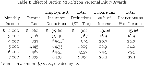
1.5 Sample calculations: In the attached table, I have calculated the impact of the Insurance Amendment Act on the loss of income claims of plaintiffs at various levels of income. In the calculation of income taxes, I have assumed that the individual has the minimum level of deductions and tax credits. Hence, the figures reported in the table should be taken as maxima. It is seen there that the effect of the Act will be to reduce awards by 15 to 25 percent.

Table 1

2. Income Tax

The Supreme Court of Canada has ruled, with respect to both fatal accident claims and claims for cost of future care, that if the annual loss is calculated net of income tax, the plaintiff is entitled to an “income tax gross-up” to ensure that the amounts available from the investment of the lump sum damages are sufficient to compensate the plaintiff for his/her future losses. As the Insurance Amendment Act does not explicitly prevent the courts from allowing a tax gross-up, it appears likely that they will allow this calculation. This means that, in every personal injury case in which the plaintiff’s damages are expected to affect his/her income for some time into the future, a tax gross-up calculation will have to be made.

2.1 The basis of the calculation: Assume that the plaintiff has lost a gross (before tax) income of $50,000 one year from now, that his income taxes on that amount would have been $10,000, and that the interest rate at which he can invest a lump-sum award is 5 percent. Prior to the passage of the Insurance Amendment Act, the plaintiff would have been entitled to an award of $47,619 – as investment of $47,619 at 5 percent will provide a return of $2,381; and $2,381 plus $47,619 is $50,000.

Under the new Act, however, the plaintiff is to be compensated only for his after-tax loss, of $40,000. Thus, if the taxes on interest were ignored, the lump-sum award would be $38,095 – as $38,095 plus 5 percent of $38,095 (= $1,905) is $40,000. However, assume that the interest on the lump sum award will be taxed at 20 percent. In that case, investment of $38,095 at 5 percent would yield a net (after-tax) return of only $1,524 ($1,905 minus 20 percent) and the plaintiff would have only $39,619 with which to replace his $40,000 loss.

The 20 percent tax on investment income has reduced the effective rate of interest by that 20 percent, from 5 percent to 4 percent. (Note that $1,524 is 20 percent less than $1,905, or 80 percent of $1,905.) Thus, if the plaintiff is to have $40,000 available to him one year from now, more than $38,095 will have to be invested today. In this case, that amount will be $38,462 – as $38,462 plus 4 percent of $38,462 (= $1,538) is $40,000. The difference between $38,462 and $38,095 is called the income tax gross-up. NOTE: The gross-up equals the income tax that must now be paid on the interest income that derives from investment of the lump-sum award.

2.2 The magnitude of the tax gross-up: Note that in my simple example, the tax gross-up was very small relative to the size of the lump sum award. This is because there was only one year of losses and, hence, the lump-sum award, (on which interest was to be calculated), was small relative to the size of the annual loss. In cases in which losses are expected to continue for longer time periods, however, both the lump-sum award and the interest earned on investment of that award will be larger relative to the size of the annual payments. In such cases, the gross-up will become a much larger percentage of the award.

For example, assume again that it has been determined that the plaintiff has lost $50,000 per year before taxes, that taxes on that income would have been $10,000 per year, and that the interest rate is 5 percent. Assume also that the loss is expected to continue for 40 years and that the lump-sum award required to replace this stream, before addition of the gross-up, would have been $500,000. If that amount is invested at 5 percent, $25,000 in interest will be generated in the first year and, at a tax rate of 20 percent, the plaintiff will be required to pay $5,000 in taxes. That $5,000, and comparable (but declining) amounts calculated in all 40 of the future years of the loss, will have to be added to the award to ensure that the plaintiff can replace his/her after-tax losses. These “additions” constitute the gross-up.

In many cases, the addition of the gross-up will increase the award by as much as half of the reduction that resulted from the omission of income taxes. For example, if the lump sum, without the gross-up, has been reduced by 20 percent, the gross-up will often add as much as 10 percent back to the award.

It is interesting to ask whether it is possible that the award with the gross-up could be higher than the award that would have resulted from application of the “old” rules, in which income taxes were ignored. The answer is that it is highly unlikely that this will occur. In the example above, the effect of the Insurance Amendment Act was to reduce the plaintiff’s annual claim by $10,000, from $50,000 to $40,000, due to the deduction of 20 percent income taxes. Before the gross-up calculation could return the lump-sum award to the level it would have had prior to the Act, the taxes on investment income – the amount to be added for the gross-up – would have to equal that $10,000. In my example, that would require that investment income be $50,000 per year as, at a tax rate of 20 percent, that would generate $10,000 worth of taxes. (For example, if the lump sum was $1,000,000 and the interest rate was 5 percent, $50,000 investment income would be generated each year.)

That is, before the tax gross-up calculation would “add back” the income tax that had been deducted as a result of the Insurance Amendment Act, (in this case, $10,000 per year), the interest income in each year would have to equal the loss of before-tax income in that year. In my example, the annual before-tax income was $50,000, on which taxes would be $10,000. In order for the investment of the lump-sum award to create $10,000 in taxes on investment income, (which is the amount to be added for the gross-up), at the same 20 percent tax rate, it would have to generate $50,000 in such income. (Again, at a 5 percent interest rate, the lump-sum would have to be $1,000,000.)

But assume that investment of the lump sum did generate $50,000 investment income. That would exactly equal the amount required to pay for both the tax on that income ($10,000) and the compensation required for the plaintiff’s loss of net income ($40,000). That is, after deduction of the two payments from the interest income, the lump-sum would be left intact. But that cannot be correct. It is clearly the intention of the court that the lump sum award be drawn down each year, to help pay for the annual losses, until there is nothing left at the end of the period of the loss. That can only occur if the investment (interest) income in each year is less than the payments for taxes and the plaintiff’s loss. And that implies that the taxes on the investment income (the gross-up) will be less than the taxes on (gross) employment income. In short, in all but very exceptional cases, the gross-up will not be sufficient to return the lump-sum to the level that would have been awarded in the absence of the Insurance Amendment Act.

3. Unanswered Questions

With respect to the income tax issue, the primary question that will have to be answered by the courts is whether a tax gross-up will be allowed. Some lesser questions may also be raised:

3.1 Collateral benefits: The Insurance Amendment Act requires that many collateral benefits be deducted from the plaintiff’s claim. It is not clear whether the plaintiff will be able to include the interest earned on the investment of such benefits in the calculation of the tax gross-up.

3.2 “Add backs”: Self-employed individuals are often able to write off personal expenses as business expenses for the purpose of calculating taxable income. For example, business owners often claim that a greater portion of their vehicle, telephone, and mortgage expenses are for business use than is actually the case. Commonly, in personal injury claims, the “personal” portions of these expenses are “added-back” to reported income in order to obtain a measure of “true” income.

How should income taxes be calculated on this “add back?” Assume, for example, that the plaintiff had been reporting earnings of $30,000 per year, on which she had been paying income taxes of $4,000. Assume also, however, that this individual had benefited personally from $5,000 worth of business expenses per year. When this amount is added back to obtain the “true” measure of income, $35,000, should the income tax calculation be based on that ($35,000) figure, even though the plaintiff had been paying taxes on only $30,000? Or should the court recognise that, in the absence of the accident, the plaintiff would have received $31,000 (= $30,000 reported income – $4,000 income tax + $5,000 “business” expenses) worth of benefits (after tax) from her employment?

3.3 Replacement cost: It is not clear how the Insurance Amendment Act will affect the determination of damages when damages are measured using the “replacement worker” method.

In many cases involving self-employed individuals it is unclear (a) what their true income would have been if they had not been injured; nor (b) what their income will be now that they have been injured. It is often possible to determine, however, how much it would cost to hire a “replacement worker” whose input would return the plaintiff’s business to its pre-injury level of profitability.

Assume, for example, that the plaintiff’s income would have been $50,000 per year if she had not been injured and that it will be $20,000 per year now that she has been injured, but that neither figure can be calculated with any degree of certainty. Assume, however, that it is known that if the plaintiff was to hire an assistant for $20,000 per year, the firm would be as profitable as it would have been if the plaintiff had not been injured. In that case, it is argued, if the plaintiff was paid $20,000 per year, she would be put back in the position she would have been in had she not been injured.

But notice, if the plaintiff had not been injured, her business would have earned a profit of $50,000 per year, on which she would have paid income taxes. With the hiring of the replacement worker, the business again makes a profit of $50,000 before payment of $20,000 to the replacement worker. But, after the replacement worker has been paid, the plaintiff’s business will show only a $30,000 profit; and it is on that number that taxes will be calculated. Thus, if the plaintiff is awarded $20,000 per year, with which to compensate the replacement worker, her net income “with injury” will be: $50,000 (= $20,000 plus $30,000) minus the taxes on $30,000. This is greater than her net income before injury, which was $50,000 minus the taxes on $50,000.

It is not clear how the court will wish to deal with this anomaly, if at all. Note that any attempt to calculate the tax implications of using the replacement worker method will require that estimates be made of both the plaintiff’s with- and without-income streams. Yet it was to avoid having to make those estimates that the replacement worker approach was devised.

4. Impact of Insurance Amendment Act

The Insurance Amendment Act will reduce damage awards by the greatest amount in the following situations:

  • Those in which the plaintiff had been earning a relatively high income and, therefore, had been paying relatively high income taxes.
  • Those in which the plaintiff’s injuries are expected to continue for a relatively long period of time, as the effect of compensating for only after-tax income will be compounded over the duration of the loss – and as the tax gross-up will not fully offset the reduction for taxes.
  • Those in which the plaintiff is not self-employed. Self-employed individuals are able to write off personal expenses against their business income. Assume that it has been determined that those expenses amount to $5,000 per year. Typically, under the current system, that $5,000 will be “added back” to reported income in order to obtain a “true” measure of income. However, the individual would have had to earn more than $5,000 in order to generate enough income to purchase $5,000 worth of goods if he/she had not been self-employed (because income taxes would have been payable on any such income). Hence, the current practice actually compensates the plaintiff only for his/her loss of after-tax income. As that is what will be required under the Insurance Amendment Act, such plaintiffs will be in the same position under this Act as they were previously.
  • Individuals who have a cost of care claim. The income tax gross-up on a cost of care claim will be higher, the greater is the award for loss of earnings. (The higher is the award for loss of earnings, the greater is the interest that will be earned on investment of that award and, therefore, the higher will be the income tax bracket in which other sources of income – for example, interest on the cost of care award – will be placed.) As the Insurance Amendment Act reduces awards for loss of earnings, it will also reduce awards for cost of care.

5. Conclusion

It is my expectation that Section 626.1(2)(a) of the Insurance Amendment Act will not introduce any significant legal principles that have not already been analysed carefully with respect to fatal accident and cost of care claims. The primary impacts of the amendments are (a) more time and effort will now have to be expended in the calculation of personal injury damages (particularly when a gross-up is required); and (b) personal injury damage awards will now be approximately 15 to 25 percent lower than they were previously.

Footnotes:

* This article is based on presentations Dr. Bruce gave to ACTLA seminars in Calgary and Edmonton on June 21 and 23, 2004. He thanks the participants at those seminars for the excellent feedback that helped him to revise his paper. [back to text of article]

leaf

Christopher Bruce is the President of Economica and a Professor of Economics at the University of Calgary. He is also the author of Assessment of Personal Injury Damages (Butterworths, 2004).

Spring 2004 issue of the Expert Witness newsletter (volume 9, issue 1)

Contents:

  • Forecasting the Rate of Growth of Real Wages (Productivity)
    • by Christopher Bruce
    • Christopher Bruce summarises the most recent theoretical and empirical evidence concerning one of the most controversial, and poorly-understood, components of the calculation of future earnings – the so-called “productivity factor.” He notes that, although the observed rate of increase in earnings is tied to the rate of increase in labour productivity over the very long run, in shorter periods the two rates may differ if there is a significant increase or decrease in the supply of labour. Specifically, he reports that most economists now believe that the slow down in “real” wage growth (the rate of growth in excess of the rate of inflation) in the 1980s and 1990s occurred because of the increase in labour supply that came with the influx of “baby boomers.” That the baby boom is now working its way through the system implies, therefore, that the rate of growth of real wages will increase significantly in the next two decades.
  • An Alternative Method for Assessing the Value of Housewife Services
    • by Douglas W. Allen
    • The article develops a new and creative method for assessing the value of the housework provided by women in “traditional” marriages; that is, by women who stay at home full time. Professor Allen is an internationally recognised expert on economic aspects of marriage and divorce. He has, for example, written extensively on the impact of no-fault divorce laws. In this article, he argues that a widely-accepted theory of the manner in which individuals choose their spouses can cast light on the implied value that couples place on the value of housework. Specifically, he notes that many theories of spousal choice predict that individuals will choose mates in such a way that the contributions of the two spouses will be equal. If this is the case, then if the husband is working in the labour market, where he earns $50,000 per year, and the wife is working only at home, the value of her contribution to the marriage must also be $50,000.

An Alternative Method for Assessing the Value of Housewife Services

by Douglas W. Allen

This article first appeared in the spring 2004 issue of the Expert Witness.

Often the simplest questions in life have the most complicated answers. Such is the case in measuring the value of non-market activity like volunteer hours, leisure time, and especially the value of a housewife. How can something so much a part of our everyday experience as “household service” be such an elusive thing to evaluate … especially in court?

Of course, at the heart of the matter is the absence of explicit market pricing for housewives. “If only,” exhorts the expert economic witness, “housewives were bought and sold on an open market like wheat futures, we could have an accurate measure of their worth.” This market oriented predilection for using prices to measure value not only drives the methods currently used, it is the source of the problems in measuring, and perhaps the source of the courts often reluctance to rely on “economic” measures of worth. To paraphrase Oscar Wilde, economists often know the price of everything, but the value of nothing.

To refresh your memory, economists have argued for two different methods to measure the value of a housewife: the opportunity cost method; and the replacement cost method.

The fundamental idea behind the opportunity cost method is “what does the household sacrifice by having the wife stay home to work?” In other words, what is the opportunity cost of the housewife’s time? If a female lawyer is earning $150/hour, and she decides to forgo an hour of work to do the dishes, the cost of that task is $150. The economist then says the $150 measures the value of an hour of housewife service.

The replacement cost approach to the problem asks: “how much would it cost to replace the services of the housewife?” The idea being one could go into the market place, find the wage for nannies, cooks, prostitutes, etc., then use these wages as the value of the housewife services. Sometimes an average is used, sometimes the wage within each specialty is used.

Both of these methods are riddled with well known problems:

  • They measure the value of household services at the margin, and not the total value.
  • The OC approach assumes your hours of work are completely flexible.
  • The RC approach assumes the productivity of the wife and market replacement are the same.
  • Both methods have a hard time dealing with full-time, long-term housewives who have been separated from the labor market for years.
  • Both methods rely on often arbitrary measures of time devoted to household services.
  • Both methods are silent on how to treat housewife services that are not available in the market.
  • Both methods have a difficult time dealing with the commingling of leisure and household services.

The list goes on. Such problems are a source of income for an expert economic witness, but there must be a better way – especially for the case of the long-term, full-time housewife where using market measures is inappropriate.

The fundamental problem with both methods is that they are based on market oriented economic theory, and as a result they ignore the institutional aspect of marriage. Marriage, as an institution, is designed to produce a set of goods that the market does not produce. Certainly some market goods get jointly produced in the marriage, but these are secondary to the main purpose of marriage. Marriage restricts the behavior of both the husband and wife such that they have an incentive over their life-cycle to cooperate in procreation and the successful rearing of the next generation. To confuse the value of a housewife with the services of domestic service misses the point entirely. The market based procedures are only crude, unreliable, and biased under-estimates of the true value of a housewife.

Within the past 25 years economists have started to move away from this purely market based way of thinking, and have started to consider the institutional aspects of exchange. This work leads to an interesting method of evaluating a housewife – one that works best in the case where the market approach does poorly. This method is simple to use, and is based on the revealed spouse choice at the time of marriage as an indicator of the value of a spouse’s contribution to a marriage.

Marriage is a sharing arrangement. A husband does not hire his wife, nor does the wife hire her husband. When the marriage is doing well both benefit, and in hard times both suffer: “for better or for worse.” Some shares are better than others. A spouse who gets a small share of the pie has little incentive to work within the marriage. The gains from an increased share to this person will more than offset the disincentives caused by reducing the share to the other spouse. Economists have shown that for a given man and woman there is an “optimal share” which creates the best incentives for the husband and wife to contribute to the marriage.

The interesting thing about the optimal share is that, with one exception, it never pays the average contribution of each spouse. For example, if one spouse were contributing 90% of the marriage value and the other spouse was contributing 10%, the optimal share turns out to always be lower than 90% for the more productive spouse. This is a good deal for the low productive spouse, but a bad deal for the partner. The only time this is not true is when each spouse is equally productive and they share 50-50.

In a marriage of unequals then, to have the optimal share means that one of the spouses is unhappy. On the other hand, to share in proportion to unequal contributions means the share is not optimal and the incentives are not right: the marriage will be low valued. In either case, there is a problem.

Couples do not marry in a vacuum. Individuals compete with one another for mates. This competition for spouses, along with the optimal sharing rule above, forces people to marry individuals they expect will make an equal contribution to the marriage. A person will always do better marrying someone of equal quality and sharing equally, rather than marry someone with of a lower quality, even though their share is higher in the latter case. The result is that in equilibrium husbands match with wives who are expected to contribute equally over the life of the marriage.

This does not mean the type of contributions are the same. The husband may be expected to work in the labor force, the wife may work in the home full time. Nor does it mean the contributions actually end up equal. It simply means that the couple believes at the time of marriage that the two different streams of services are of equal value – otherwise they wouldn’t marry. Thus this approach recognizes the most valuable contribution of a full-time housewife – giving birth and raising children. The other methods, by focusing on simple household chores, ignore the most important contribution of the wife.

Recognizing the incentives of sharing within a marriage explains why marriages have a hard time surviving large unexpected shocks like infertility or long spells of unemployment. An option to divorce is to renegotiate the share. However, renegotiation, ex post, will always imply a sub-optimal share. The spouse who ends up, ex post, more productive will always be better off finding a new mate of similar productivity.

Recognizing the incentives of sharing explains why full time working wives still tend to do more than half of the housework in a marriage. Women still earn 70% of men, on average. Since total contributions must be equal in successful marriages, women who contribute less market value to the marriage must contribute more household services.

The idea that people tend to marry equals is in our popular culture. The expression “what does she see in him?” indicates that some hidden redeeming feature must be present to compensate for an observable shortcoming.

If we accept the argument that individuals marry others of equal expected value, then we have a simple, but better, method of measuring the value of household services for marriages that remain intact. If a marriage is on-going, the partners must feel that on average they are getting out of the marriage what they are putting in, and that this marriage provides a higher value than marriages to other people. The condition for this is that the partners are making approximately equal contributions and are sharing 50-50. Thus, to determine the value of household services we need only look at the market earnings of the husband and adjust for the market earnings of the wife, and the household services of the husband. Or:

Value of housewife = Husband’s incomeWife’s income + value of husband’s household services.

Suppose the wife does not work outside the home, and the husband never does any work around the house. Then the value of the wife’s household service is simply equal to the husband’s income. This methodology is not only easier than the standard ones, it is better in that it is a true measure of value, rather than just cost. It is better because it does not have any of the ad hoc aspects of the market measures since it relies on the revealed behavior of the individuals to assess their own value.

leaf

Douglas W. Allen is the Burnaby Mountain Endowed Professor of Economics, Department of Economics, Simon Fraser University

Forecasting the Rate of Growth of Real Wages (Productivity)

by Christopher Bruce

This article first appeared in the spring 2004 issue of the Expert Witness.

One of the most important determinants of the value of an individual’s lifetime income is the rate
at which that income will grow from one year to the next. The lifetime income of an individual whose earnings grow at 1 percent per year will be dramatically lower than that of an individual whose earnings grow at 5 percent per year. Two major factors determine this growth rate, once the individual has chosen an occupation. First, as workers obtain more experience, their earnings increase due to what is often called
“career progress.” Second, all workers in society tend to benefit equally from the long-term rise in wages across the economy. (If average wages rise by 50 percent over a period two decades, we expect that the wages of labourers and waitresses will increase by 50 percent also, even if the skills required for those two jobs remain unchanged.2)

Furthermore, economy-wide wage increases can be divided into those that are due to changes in the consumer price index – inflationary increases – and those that are due to changes in the “real” purchasing power of wages – real wage increases. (The observed, or “nominal,” rate of increase of wages equals the rate of price inflation plus the rate of increase of real wages.) Unfortunately, despite its importance for the calculation of damages, the forecast of real wage increases proves to be very complex. The purpose of this article will be to report some recent developments in the preparation of that forecast that should prove to be valuable to the courts.

Introduction

Effectively, an increase in the real wage is an increase in the purchasing power of workers’ earnings. But, in the
long run, the average worker will only be able to consume more goods and services if output per worker has increased. Therefore, one would expect there to be a correlation between the long run rate of growth of real wages and the rate of growth of (real) output per worker, or “labour productivity.”

Depending upon the purpose to which it is to be put, a number of different definitions of labour productivity have been proposed. The definition that is most relevant to the determination of real wages is output per hour worked. Changes in this measure are influenced by three factors: increases in the amount of capital goods (machinery, buildings, computers, etc.) per worker, improvements in the technology “embodied” in capital (technological change), and changes in the productivity of workers (usually attributed to improvements in education).

Theory

Because a portion of any change in output per worker is attributable to changes in the quality and quantity of the capital available to workers, some of that increase in output will be paid to the owners of capital. Recently, most economists have come to accept the view that the allocation of gains between capital and labour will be determined in large part by the relative scarcity of those two factors.3 That is, in periods in which labour is in short supply (relative to capital), workers will be able to capture most of the gains from increased productivity and the percentage increase in real wages will equal or exceed the percentage increase in productivity. Conversely, when capital is in short supply relative to labour, it is capital that will capture most of the gains.

One of the attractive features of this theory is that it helps to explain many of the movements in real wages and labour productivity that have been observed over the last five decades. In the 1950s and 1960s, when the economy was growing rapidly and labour was (relatively) in short supply, real wages rose quickly, and at a rate higher than the rate of increase of output per worker. In the 1970s and 1980s, however, when the baby boom generation began to enter the labour market, labour supply increased significantly. Furthermore, because young adults borrow heavily – to purchase homes, cars, furniture, etc. – the influx of young baby boomers drove up interest rates, impeding firms’ ability to borrow for investments in capital. As a result, real wages stagnated even though productivity rose steadily. In the latter half of the 1990s, however, the baby boomers began to approach retirement age. Not only did the supply of labour start to fall, but older workers began to accumulate retirement savings, making funds available for capital investments. The result is that labour has become scarce relative to capital; and economists are now predicting that increases in real wages will begin to match, or exceed, the growth in output per worker.

Empirical evidence

Many economists believe that the reversal in the relative scarcities of labour and capital began in the mid-1990s. Some evidence in support of this conclusion is provided in Table 1. There it is seen that, between 1990 and 1995, the real incomes of Canadian males (25-44 years old, working full-time, full-year) decreased by 0.8 percent per year. (Nominal incomes increased by 1.4 percent per year during that period, while inflation averaged 2.2 percent.) However, between 1995 and 2000, average incomes increased by 3.1 percent while inflation was 1.7 percent, resulting in real income growth of 1.4 percent per year. Table 1 also reports that the real incomes of university graduates grew at 1.7 percent per year in the late 1990s; and that those of high school graduates and holders of trades diplomas and certificates made modest, but positive, gains in that same period.4

Table 1

Most Canadian economists appear to believe that, over the long run, output per worker will increase at between 1.5 and 2.0 percent per year. The 2.0 percent forecast is the consensus prediction of a group of Canada’s leading academic and government economists.5 The lower predictions have been made by forecasting agencies: Global Insight has forecast 1.9 percent per year over 2002-26; Informetrica has forecast 1.6 percent over the same period; and the Conference Board of Canada has forecast 1.46 percent over 2002-15.6Thus, as the model described above suggests that real wages will increase more rapidly than productivity, as the baby boomers age, a conservative estimate would be that real wages will increase by 2 percent per year over the next two decades.

>Conclusion

It is important to note that this means that all workers’ real wages will increase by 2 percent per year. Economy-wide productivity gains are like a rising tide, they carry all workers with them equally. Even the individual who remains in the same job, with no personal increase in productivity and no promotions, can expect, on average, to benefit from real wage increases of 2 percent per year. With inflation predicted also to be 2 percent per year, he or she is predicted to benefit from nominal wage increases of approximately 4 percent per year – a 2 percent inflationary increase plus a 2 percent real increase.

Footnotes:

1. This discussion is taken from Chapter 5 of Christopher Bruce, Assessment of Personal Injury Damages, 4th Edition, Butterworths, 2004.[back to text of article]

2. Evidence that all wages in the economy rise together, regardless of differences in the rate of increase of productivity among industries, was provided by Christopher Bruce in The Connection Between Labour Productivity and Wages (The Expert Witness Vol. 7, No. 2).[back to text of article]

3. See, especially, J. C. Herbert Emery and Ian Rongve, “Much Ado About Nothing? Demographic Bulges, the Productivity Puzzle, and CPP Reform,” Contemporary Economic Policy, 17 January 1999, 68-78; Henning Bohn, “Will social security and Medicare remain viable as the U.S. population is aging?” Carnegie-Rochester Conference Series on Public Policy 50 1999, 1-53; and William Scarth, “Population Aging, Productivity and Living Standards;” in Andrew Sharpe, France St.-Hilaire, and Keith Banting, eds. The Review of Economic Performance and Social Progress 2002, Institute for Research on Public Policy, Montreal, 2002, 145-156.[ back to text of article]

4. U.S. data also suggest that there was a striking switch to a high productivity growth regime in the mid-1990s. See, for example, James Kahn and Robert Rich, “Tracking the New Economy: Using Growth Theory to Detect Changes in Trend Productivity,” Staff Reports, Federal Reserve Bank of New York, No. 159, January 2003.[ back to text of article]

5. Andrew Sharpe,
“Symposium on Future Productivity Growth in Canada: An Introduction,” International Productivity Monitor, 7, Fall 2003, 44-45.[ back to text of article]

6. These figures are taken from Andrew Sharpe, ibid. pp. 44-45.[ back to text of article]

leaf

Christopher Bruce is the President of Economica and a Professor of Economics at the University of Calgary. He is also the author of Assessment of Personal Injury Damages (Butterworths, 2004).

Economica’s Privacy Policy

by Christopher Bruce

On January 1, 2004 the federal Personal Information Protection and Electronic Documents Act was extended to every organization that collects, uses or discloses personal information in the course of a commercial activity within a province. On the same date Alberta’s Personal Information Protection Act came into effect. The purpose of the (Alberta) Act is to “govern the collection, use and disclosure of personal information by organizations” (see www.psp.gov.ab.ca/faq.html). In light of these events, we outline Economica’s privacy policy:

  • We do not reveal any information concerning the specifics of any case, including the names and personal circumstances of the litigants, to any party other than the law firm that has retained us – unless that firm has specifically requested that we do so. We will not, for example, provide copies of our reports to the plaintiff or defendant, to any other expert who has been retained in the litigation at hand, or to any other law firm that is involved in the litigation without a specific request by the firm that has retained us.
  • All of the documents that we receive concerning the specifics of a case are kept in secure areas and/or in secure computer files. All such documents will be maintained in such a manner that they are not accessible to casual observation by visitors to our offices.
  • We will not discuss a case with any party other than the firm that has retained us, without previously having received the permission of that firm. We will not, for example, request personal information from the plaintiff, the plaintiff’s family, or the plaintiff’s employer, or from other experts without first informing the firm that retained us.
  • When speaking with third parties, such as employers, we will not reveal the name or circumstances of the plaintiff unless it is necessary to do so. If, for example, it is possible to obtain details concerning the plaintiff’s pension plan from his/her employer without revealing the plaintiff’s name, we will do so.
  • When disposing of confidential files concerning any litigant, we will have those files shredded by a professional firm.

leaf

Christopher Bruce is the President of Economica and a Professor of Economics at the University of Calgary. He is also the author of Assessment of Personal Injury Damages (Butterworths, 2004).