Winter 2000 issue of the Expert Witness newsletter (volume 5, issue 4)

Contents:

  • Incorporating the Effect of Reduced Life Expectancy into Awards for Future Costs of Care
    • by David Strauss, Robert Shavelle, Christopher Pflaum, & Christopher Bruce
    • In this article David Strauss, Robert Shavelle, Christopher Pflaum, and Christopher Bruce argue that the method used by most economists and actuaries for calculating life expectancy among the seriously disabled is flawed. They argue that this method leads to the systematic overestimation of costs of future care. They show, for example, that the costs of care for plaintiffs with cerebral palsy are commonly overestimated by 10 to 15 percent. Strauss and Shavelle are able to provide life expectancy data that correct for this error.
  • Evaluation of Harm to a Class of Individuals
    • by Kelly Rathje
    • In this article Kelly Rathje explains how the estimates of damages can be improved if the plaintiff is one of a class of individuals who have been affected by the same harm. In such cases, a statistical technique known as econometrics can be employed to compare the earnings capacity of the victims of the harm with the earnings capacity of a randomly selected sample of individuals who have not been so-harmed. This technique can be used, for example, to determine the impact of sexual abuse on a students at an orphanage or residential school.
  • What is Econometrics?
    • by Kelly Rathje and Christopher Bruce
    • In this article Chris Bruce and Kelly Rathje explain the fundamental principles of “econometrics”.

What is Econometrics?

by Kelly Rathje & Christopher Bruce

This article was originally published in the Winter 2000 issue of the Expert Witness.

Commonly, economic experts will testify that a particular characteristic of the plaintiff, such as his years of education or his marital status, is “correlated” with one of the factors that is of interest to the court, such as future income or retirement age. The branch of economics that seeks to determine whether such correlations exist is called econometrics. In this article, we explain briefly how econometric techniques work.

Assume that we are interested in determining whether the annual incomes that individuals earn are correlated with, or determined by, years of education. Assume also that 70 individuals have been observed and that for each individual, we know their number of years of education and annual income.

We have plotted the observations for these individuals in Figure 1. For example, individual A has 15 years of education and an annual income of $45,000.

Figure 1

When income levels are plotted against years of education, one would expect that the observations would be scattered, as seen in Figure 1. What the econometrician wishes to do is determine whether these scattered points form a “pattern.” One simple pattern that is often tested is that of a straight line. In this case, the formula for a straight line is:

I = a + b1(E)

where I is income; a is a constant; b1 measures the amount that education influences income; and E is years of education.

What the econometrician tries to do is to find the line which minimises the distances between the observations and the points on that line. The straight line which appears to meet this criterion with respect to the observations in Figure 1 has been drawn there. The formula for this line is

I = 6,850 + 2,000(E) (1)

This formula says that if the individual has 12 years of education, his income is predicted to be $30,850.

I = 6,850 + 2,000(12) = 30,850

It can be seen from Figure 1 that, in general, the observations lie fairly close to the line. For this reason, we would conclude that the hypothesis that education affects income is supported. Furthermore, because the “sign” on the 2,000 component of the equation is positive, we would also conclude that education has a positive effect on income. (In this case, each extra year of education appears to lead to 2,000 extra dollars of annual income.)

Equation (1), which investigates the effect which only one variable has on another, is not typical of the equations that are normally of interest to economists. Typically, for example, we would assume that there is a large number of factors, in addition to education, that will affect income. In that case, econometricians extend their equations to include numerous variables.

For example, suppose the economist has additional information about the age of each individual in the data set. This variable can also be added to the equation to help “explain” income. The equation would become:

I = a +b1(E) + b2(A),

where A is “age.” The resulting estimated equation might be something like:

I = 5,000 + 1,900(E) + 200(A) (2)

This model now indicates that for every extra year of education an individual has, they will earn an extra $1,900, on average, and for each additional year in age, there is an increase of $200. In other words, if an individual has a high school diploma, and is 34 years old, then the equation indicates on average, they will earn $34,600 (= 5,000 + [1,900 x 12] + [200 x 34]). Similarly, if an individual holds a bachelor’s degree (16 years of education), and is 34 years old, then the equation indicates that, on average, they will earn $42,200 (= 5,000 + [1,900 x 16] + [200 x 34]).

The variables used as examples to this point – income, education, and age – all share the characteristic that they can easily be measured numerically. Other variables which might influence the wage rate are less easily converted to numerical equivalents, however. Assume, for example, that our hypothesis was that incomes were higher in rural areas than in cities, or that men were paid higher incomes than women, all else being equal.

As econometric analysis is a statistical technique, it requires that the economist enter all of his or her information as numbers. The way that econometricians deal with this problem is to construct what are called “dummy variables.”

In this procedure, one of the observations is arbitrarily chosen to be the “reference variable” and it is given the value of 0 whenever it appears. The other observation is then given the value of 1. For example, if “female” was the reference category, then the dummy variable would be given the value 0 whenever the observed individual was female and would be given the value 1 whenever the individual was male.

Assume that this has been done and equation (2) has been re-estimated with a male/female dummy variable included. The new equation might look like:

I = 3,000 + 1,900(E) + 200(A) + 4,000(M) (3)

where M is 1 if the individual is male and 0 if she is female. The interpretation that is given to the value that appears in front of M in this equation is that income is $4,000 higher when the worker is a male than when the worker is female.

Alternatively, because the dummy variable takes on the value 0 when the worker is female, the relevant regression equation for females is simply equation (3) excluding the dummy variable:

I(female) = 3,000 + 1,900(E) + 200(A)

And because the dummy variable takes on the value 1 when the worker is male, the relevant equation for males becomes:

I(male) = 3,000 + 1,900(E) + 200(A) + 4,000(1)

= 7,000 + 1,900(E) + 200(A)

The income model is one example of how econometrics is used, and how it is useful to determine trends and relationships between variables. Other uses may include forecasting prices, inflation rates, or interest rates. Econometrics provides the methodology to economists to make quantitative predications using statistical data.

leaf

Kelly Rathje is a consultant with Economica and has a Master of Arts degree (in economics) from the University of Calgary.

Christopher Bruce is the President of Economica and a Professor of Economics at the University of Calgary. He is also the author of Assessment of Personal Injury Damages (Butterworths, 2004).

Evaluation of Harm to a Class of Individuals

by Kelly Rathje

This article was originally published in the Winter 2000 issue of the Expert Witness.

When we are asked to estimate a claimant’s potential future income (without- or with-accident) we rely on two types of data – data specific to the individual, such as the claimant’s tax returns, and statistical data concerning individuals “similar” to the plaintiff, such as information drawn from the Census.

When the plaintiff is part of a common class of victims, however, it is possible to rely on more sophisticated statistical techniques to assess the impact of the injurious act. Such classes of plaintiffs might include, for example, victims of chemical or radiation poisoning in a factory or residential area or victims of sexual or physical abuse at a school.

In these cases, economists can rely on a technique known as econometric modelling (see the accompanying article from this newsletter) to determine whether the average income of the class of victims differs significantly from the average income of a similar group chosen at random from the population.

The difference may be determined by specifying characteristics, common to both groups, and examining how these factors influence income. Any difference in income not attributable to the specified characteristics could be attributed to the incident, and thus the loss of income due to the incident may be determined.

To use this method, an economist would need to gather data, do some comparative statistical analysis, and then apply the econometric model. These steps are outlined below.

Data

The data for the claimant’s group is most commonly compiled from information provided by the individuals within that group. The comparison group, which is to represent a random sample from the population, can often be obtained from broad data sources such as the census.

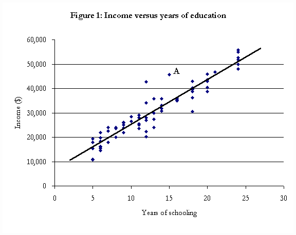
Using these sources, the economist would create two types of variables. The first of these are “numerical” variables; that is variables that can be measured using numerical scales. For example, if the economist is trying to identify the determinants of income, numerical variables might include age, years of education, and work experience.

The second set of variables, “dummy” variables, are variables that cannot be measured numerically. For example, these might include place of residence or sex of the individual. For example, if the economist wished to test the hypothesis that people in the Maritimes earned less than individuals in the rest of Canada (ROC), a variable might be created that divided the group between Maritimes and ROC.

Comparisons

Before any formal estimation is done, economists usually look at the raw data to see if any trends or relationships are present. Using the characteristics indicated above (age, place of residence, years of education, and current income), trends of interest to economists might be employment rates, average numbers of years of educational attainment, and average income levels for each group.

Econometric modelling

Using the characteristics outlined, an (econometric) equation is created to examine the factors that influence income. The equation, in its simplest form, might be as follows:

I = C + b1[age] + b2[maritimes] + b3[claimants]

What this equation predicts is that income, I, will be determined by the individual’s age, place of residence, membership either in or out of the “claimant” group, and a fixed factor, C. In this equation, “age” is a numerical variable – it might take values such as 25 or 47 years old, for example.

“Maritimes” and “claimants” are dummy variables. In this case, “Maritimes” takes the value 1 if the individual lives in the Maritimes and 0 if he or she lives in the ROC; and “claimants” takes the value 1 if the individual is one of the plaintiffs and 0 if he or she was chosen from the random sample of other individuals in the population.

Once the data set has been collected, and the form of the equation has been identified, statistical techniques are applied to the data to estimate the “best” values of b1, b2, and b3.

The data might suggest, for example, that the most likely relationship among the variables is:

I = 25,000 + 500[age]- 4,500[maritimes] – 20,000[claimants]

This indicates that for each year an individual ages, income increases by $500, on average; and that if the individual lives in the Maritimes, income will be, on average, $4,500 less than if that individual lives in the ROC. The above estimation also indicates that, on average, the claimant group will earn $20,000 less than average individuals in the population, all else being equal. For example, a 37-year-old, who lives in the Maritimes, and is not part of the claimant’s group would earn $39,000 (= 25,000 + 500[37] – 4,500[1] – 20,000[0]); and a 37-year-old, who lives in the Maritimes, and is a part of the claimant’s group would earn $19,000 (= 25,000 + 500[37] – 4,500[1] – 20,000[1]);

Now suppose the economist also has information on the employment status of each individual in both groups. The next step that may be undertaken is to estimate what an individual’s income would be given the above characteristics, but limiting the observations to employed individuals only. That is, the economist might control for employment status by including only observations at which the income is greater than zero. This would indicate how much of the difference in income, found in the first estimation, could be attributed to employment status. The resulting equation might be, for example:

I = 21,000 + 200[age] – 4,500[maritimes] – 12,000[claimants]

Given that I > 0

Recall from above, when considering both employed and unemployed individuals together, the equation indicated that the claimant’s group earned approximately $20,000 less than the random population. Now, controlling for employment, they are found to earn $12,000 less. This implies that $8,000 of the earnings gap between the plaintiff group and the general population can be explained by the higher unemployment rate of the former group.

Now suppose there is additional information regarding the education levels of the groups. The next logical step would be to add educational attainment as one of the explanatory variables. Thus, the equation would include the number of years of education, place of residence, age, and “claimant” status. This specification adds another explanatory factor to help predict income levels. Still controlling for employment status, the resulting equation might be:

I = 20,000 + 100[age]- 4,000[maritimes] + 2,000 [education] – 7,000[claimants]

Given that I > 0

This equation, given the known characteristics in this example, has the most explanatory power. It indicates to the economist that controlling for all the known variables, there still exists a difference in income of $7,000 between the claimants and an individual chosen at random from the general population, given that both individuals have the same characteristics.

Note, however, that this does not mean that the effect of the tortious act is, on average, $7,000 per year per claimant. First, remember that when no allowance was made for employment status or education, the average difference between the annual incomes of the claimants and members of the general population was $20,000. What the last equation predicts is that if we compare two individuals who have the same education and the same employment status, we will find that the “claimant” earns, on average, $7,000 less than the non-claimant. However, the effect of the tortious act may have been to increase the unemployment rates of the claimants and reduce their educational attainments (particularly if they were injured while they were minors). In that case, the $7,000 would represent the lower bound on the estimated impact of the injury.

Second, part of the income differential between claimants and non-claimants may be the result of factors that have not been taken into account in the equations. For example, assume that the claimants had all been harmed by the release of a toxic chemical. It might be that individuals who are susceptible to that chemical share some genetic factor that also reduces their abilities to earn income. If that genetic factor is not taken into account, the statistician may attribute the lower incomes of members of that group to the chemical when, in fact, that group would have earned lower incomes in any event.

Another drawback is that this method determines average incomes for the group, and thus, average differentials for the group. That is, the income differentials between the claimant group and the random group apply to the overall group, and not necessarily to each claimant. When the claimants are considered individually, the economist may find that some of the claimants are earning more than the average income predicted by the model; some are earning less income than the average income predicted by the model; and some are earning the same income the model predicted. However, on average, the group still has a reduction in earnings, when compared to individuals chosen at random from the population, with the otherwise same characteristics (other than the incident).

We were recently asked to determine whether there was economic evidence to support a claim that a group of individuals experienced a loss of income as a result of a common incident. We followed much of the same steps and methodology described here in determining: (i) whether an income differential existed; and (ii) the extent to which each of the known factors influence income. This methodology allowed a quantitative measure of the loss of income to be predicted, given the information provided by the group, and compared to a random sample of the population.

leaf

Kelly Rathje is a consultant with Economica and has a Master of Arts degree (in economics) from the University of Calgary.

Incorporating the Effect of Reduced Life Expectancy into Awards for Future Costs of Care

by David Strauss, Robert Shavelle, Christopher Pflaum, & Christopher Bruce

This article was originally published in the Winter 2000 issue of the Expert Witness.

1. Introduction

Some of the largest personal injury and medical malpractice actions are brought on behalf of plaintiffs with chronic disabilities such as cerebral palsy, spinal cord injury, and traumatic brain injury. Such plaintiffs require extensive care and assistance for the rest of their lives, and the cost of future care is often the largest part of the claim.

There are three components to the calculation the present value of the cost of lifetime care:

  1. A discount rate, specifying the interest rate at which it is assumed the lump sum award will be invested.
  2. The dollar cost of providing care during each year. The rate at which this amount is assumed to grow over time is usually, though not necessarily, lower than the rate of discount.
  3. A probability distribution specifying the probability that the plaintiff will live to each possible age in the future. In the calculation of the present value of future costs of care, the cost of care in each possible year in the future is multiplied by the probability that the individual will live to the age at which that cost is required. This is equivalent to reducing the required cost by the probability that the plaintiff will not live to a given age and, therefore, that the plaintiff will not require the assumed cost of care. [Note that this is analogous to multiplying the annual loss of income by the probability that the individual would have been working during that year, in order to capture the effect of the probability that the individual would have been unemployed.]

When the injury is not one that reduces life expectancy, the survival distribution that is used is that of the general population. The distribution can be obtained from an ordinary life table. (In Canada, this is the Life Tables 1990-1992.) Our interest here, however, is the case in which life expectancy is reduced, and it is no longer obvious how the annual survival probabilities should be chosen.

2. Alternative methods of calculating the impact of reduced life expectancy

Typically, medical opinion concerning reduced life expectancy is conveyed in the form of an average number of years of expected survival. For example, the medical experts might agree that the effect of the plaintiff’s injury is to reduce her life expectancy from 50 years to 30. The question we wish to consider here is how economists should incorporate this opinion in their calculation of the changes in annual probabilities of survival. A number of alternative techniques are commonly used.

Life certain – A very simple technique is to assume that the plaintiff will live exactly the number of years estimated by the medical experts and then die. For example, a 30 year-old who has a probability of 1.0 of living to each age between 30 and 50, and a probability of zero of living to any age beyond that, has a life expectancy of 20 years.

Although this technique is sometimes used to obtain to obtain very rough approximations, it is certain to produce estimates that exceed the true value by a substantial amount. The reason for this is that the life certain approach leaves all of the costs of care in the immediate future, (in this case, in next 20 years). In reality, the plaintiff has some probability of dying during the next 20 years and a corresponding probability of living more than 20 years. Hence, in reality, the costs of care should be reduced in the near future (to allow for the possibility that the plaintiff will die before needing them) and increased in the distant future (to allow for the possibility that the plaintiff will live beyond 20 years). But, as discounting reduces the present value of ‘distant’ costs more than it reduces the present value of ‘near’ costs, moving costs further into the future will reduce the discounted value of future costs.

Rating up – A simple method for obtaining a probability of survival to each possible age in the future is to find a “statistical person” who has the life expectancy of the injured plaintiff and to use that person’s probability distribution to represent that of the plaintiff. For example, consider a boy with severe cerebral palsy who has an agreed upon life expectancy of 20 additional years. The rating up method identifies the age in the general population at which the life expectancy is likewise 20 years.

According to the U.S. Decennial life tables, for example, this is 58 years. For each future age, the probability of survival for a 58 year old is substituted for that of the 5 year old. For example, the 5 year-old’s probability of living to age 15 is assumed to equal the probability that an average 58 year old would live to 68.

The attraction of this method is that it provides a probability distribution with the correct average, (here, 20 years). There is a problem, however: it is the wrong distribution. As the research literature makes clear, a child with a short life expectancy is subject to a fairly constant risk over the life span; he may well die in the next few years but he also has a reasonable chance of living another fifty. By contrast, the man of age 58 is at a relatively low risk over the next few years, but his risk increases steeply over the decades and he has almost no chance of surviving another 50 years.

Like the life certain method, the rating up method places too many of the costs of care in the immediate future, and too few in the distant future (relative to the “true” values). Hence, it systematically overestimates the present value of future costs of care.

Relative risk – In this approach, the economist multiplies all the age-specific mortality rates in a standard life table by a constant. The constant is chosen to result in the desired life expectancy, and is easily determined by trial and error. For example, if the annual probabilities that a male will die are multiplied by 47, the life expectancy of a 5 year-old will become 20 years. Although the argument is more complex than that made with respect to rating up, the relative risk approach also systematically overestimates the present value of future costs.

3. An Example

Table 1 shows lump sum awards for a 5 year-old boy with life expectancy 20 years who is to receive $100,000 for each remaining year of life. A discount rate of 4 percent is employed.

Table 1

The first row applies to a hypothetical child who will survive exactly 20 more years. This is the life certain distribution discussed above, and it leads to the largest award: $1,413,394. The second row is the result of rating up to age 58, which currently, perhaps, is the most widely used approach. The award of $1,296,174 is appreciably smaller than the $1,413,394 of row 2.

Row 3 uses the relative risk method. As indicated above, when the mortality rates of a standard life table are multiplied by 47, the life expectancy for a boy of age 5 years becomes 20 years. This is the multiplier that has been used. The resulting award of $1,297,290 is very similar to that obtained from rating up. Finally, row 4 gives the award when the correct life table, based on the latest evidence concerning cerebral palsy, is used. Use of the correct probability distribution leads to an award of $1,147,979.

In this example, both rating up and the relative risk method lead to awards that are too high by 13 percent, or approximately $150,000. And the life certain method leads to an award that is too high by almost 25 percent.

4. Comparison of the methods

The size of the discrepancy between the approximate methods and the correct survival distribution depends on several factors, of which the most important are the cost schedule, the discount rate, and the plaintiff’s life expectancy. Discrepancies will tend to increase as the rate of growth of costs decreases, as the discount rate increases, and as post-injury life expectancy falls.

Tables 2 and 3 show the percentage overestimation for various discount rates with the rating up and relative risk methods, respectively. In addition to the case of a five year old with cerebral palsy (Tables 2a and 3a), we also consider that of a 25 year-old with traumatic brain injury and a life expectancy of 20 years (Tables 2b, 3b). As expected, the amount of overestimation decreases as the net discount rate (the discount rate minus the rate of growth of costs of care) decreases, and is negative when the net rate is negative.

Table 2

Table 3

5. Conclusion

To calculate the present value of the lifetime care of a disabled person we need more than a life expectancy – the whole life table is needed. We have seen that rating up and other approximate methods can lead to substantially different present values from the values derived from the correct life table. In the common case of positive net discount rates, the approximate methods systematically overestimate the correct values. These overestimates can often amount to more than $100,000. This is an issue that has received far less attention from the courts than it deserves.

leaf

David Strauss, Ph.D., FASA, and Robert Shavelle, Ph.D., MBA, are the principals in Strauss & Shavelle, a San Francisco firm that specialises in calculation of life expectancy.

Christopher Pflaum, Ph.D., owns Spectrum Economics, an Overland Park, Kansas firm specialising in the calculation of personal injury damages.

Christopher Bruce is the President of Economica and a Professor of Economics at the University of Calgary. He is also the author of Assessment of Personal Injury Damages (Butterworths, 2004).